CNV seq

Here we show an implementation of CNV-seq

Step - 1 This includes generating best-hit location files for each mapped sequence read. The authors provide a perl script for BLAT psl file and SOLiD maching pipeline. For BAM files, they suggest to extract locations using the following command

~/copynumber$ samtools view -F 4 tumorA.chr4.bam |perl -lane 'print "F[2]\t$F[3]"' >tumor.hits

~/copynumber$ samtools view -F 4 normalA.chr4.bam |perl -lane 'print "F[2]\t$F[3]"' >normal.hits

Step - 2 cnv-seq.pl is used to calculate sliding window size, to count number of mapped hits in each window, and to call cnv R package to calculate log2 ratios and annotate CNV

perl cnv-seq.pl --test tumor.hits --ref normal.hits --genome human

two output files are produced. They can be found under "result files": < a href ="https://raw.github.com/Bioconductor/copy-number-analysis/master/result%20files/tumor.hits-vs-normal.hits.window-10000.minw-4.cnv">tumor.hits-vs-normal.hits.window-10000.minw-4.cnv < a href ="https://raw.github.com/Bioconductor/copy-number-analysis/master/result%20files/tumor.hits-vs-normal.hits.window-10000.minw-4.count"> tumor.hits-vs-normal.hits.window-10000.minw-4.count

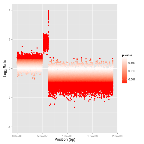
Step - 3 One can visualize the cnv inside R using the following code snippet the plot can be found under "image" folder ![] (https://raw.github.com/Bioconductor/copy-number-analysis/master/image/cnv-seq-plot.png)

The R code for visualizing the plot can be found at : CNV-seq.R