Implementation of piecewise structural equation modeling (SEM) in R, including estimation of path coefficients and goodness-of-fit statistics.
A formal description of this package can be found at:
Lefcheck, Jonathan S. (2015) "piecewiseSEM: Piecewise structural equation modeling in R for ecology, evolution, and systematics." Methods in Ecology and Evolution. In press. DOI: 10.1111/2041-210X.12512
Version: 1.0.4 (2016-02-09)
Author: Jon Lefcheck [email protected]
Supported model classes include: lm, glm, glm.nb, gls, pgls, lme, glmmPQL, and merModLmerTest.
##Examples
###Load package
# Install latest version from CRAN
install.packages("piecewiseSEM")

# Install dev version from GitHub
# library(devtools)
# install_github("jslefche/piecewiseSEM")

library(piecewiseSEM)
###Load data from Shipley 2009
data(shipley2009)
The data is alternately hosted in Ecological Archives E090-028-S1 (DOI: 10.1890/08-1034.1).
###Create model set
The model corresponds to the following hypothesis (Fig. 2, Shipley 2009);
Models are constructed using a mix of the nlme and lmerTest packages, as in the supplements of Shipley 2009.
# Load required libraries for linear mixed effects models
library(lmerTest)
library(nlme)

# Load example data
data(shipley2009)

# Create list of models corresponding to SEM
shipley2009.modlist = list(

  lme(DD~lat, random = ~1|site/tree, na.action = na.omit,
  data = shipley2009),

  lme(Date~DD, random = ~1|site/tree, na.action = na.omit,
  data = shipley2009),

  lme(Growth~Date, random = ~1|site/tree, na.action = na.omit,
  data = shipley2009),

  glmer(Live~Growth+(1|site)+(1|tree),
  family=binomial(link = "logit"), data = shipley2009)

  )
###Run Shipley tests
sem.fit returns a list of the following:
(1) the missing paths (omitting conditional variables), the estimate, standard error, degrees of freedom, and associated p-values;
(2) the Fisher's C statistic, degrees of freedom, and p-value for the model (derived from a Chi-squared distribution);
(3) the AIC, AICc (corrected for small sample size), the likelihood degrees of freedom, and the model degrees of freedom.
The argument add.vars allows you to specify a vector of additional variables whose causal independence you also wish to test. This is useful if you are comparing nested models. Default is NULL.
The argument adjust.p allows you to adjust the p-values returned by the function based on the the total degrees of freedom for the model (see supplementary material, Shipley 2013). Default is FALSE (uses the d.f. reported in the summary table).
(See "p-values and all that" for a discussion of p-values from mixed models using the lmer package.)
sem.fit(shipley2009.modlist, shipley2009)

# $missing.paths
#  missing.path     estimate  std.error   DF crit.value   p.value
#   Date <- lat -0.009051378 0.11347661   18     -0.080 0.9373049
# Growth <- lat -0.098862826 0.11072020   18     -0.893 0.3836896
#   Live <- lat  0.030497018 0.02966210   NA      1.028 0.3038804
#  Growth <- DD -0.010613707 0.03576722 1329     -0.297 0.7667083
#    Live <- DD  0.027190386 0.02708834   NA      1.004 0.3154908
#  Live <- Date -0.046565402 0.02981190   NA     -1.562 0.1182942
#
# $Fisher.C
# fisher.c  k p.value
#    11.54 12   0.484
#
# $AIC
#   AIC   AICc  K    n
# 49.54 50.079 19 1431
The missing paths output differs from Table 2 in Shipley 2009. However, running each d-sep model by hand yields the same answers as this function, leading me to believe that updates to the lme4 and nlme packages are the cause of the discrepancy. Qualitatively, the interpretations are the same.
###Extract path coefficients
Path coefficients can be either unstandardized or standardized (centered and scaled in units of standard deviation of the mean, or scaled by the range the data). Default is none. The function returns a data.frame sorted by increasing significance.
sem.coefs(shipley2009.modlist, shipley2009)

#   response predictor   estimate   std.error      p.value
#       Date        DD -0.4976475 0.004933274 0.000000e+00
#     Growth      Date  0.3007147 0.026631405 2.670862e-28
#       Live    Growth  0.3478541 0.058404201 2.585211e-09
#         DD       lat -0.8354736 0.119422385 1.565614e-06

sem.coefs(shipley2009.modlist, shipley2009, standardize = "scale")
###Generate variance-covariance SEM using lavaan
Generate variance-covariance based SEM from the list of linear mixed models. The resulting object can be treated like any other model object constructed using the package lavaan.
(lavaan.model = sem.lavaan(shipley2009.modlist, shipley2009))

# lavaan (0.5-18) converged normally after  27 iterations
#
#                                                   Used       Total
#   Number of observations                          1431        1900
#
#   Estimator                                         ML
#   Minimum Function Test Statistic               38.433
#   Degrees of freedom                                 6
#   P-value (Chi-square)                           0.000
The output shows that the variance-covariance SEM is a worse fit, indicating that a hierarchical piecewise approach is justified given the hierarchical structure of the data.
###Plot partial effect between two variables
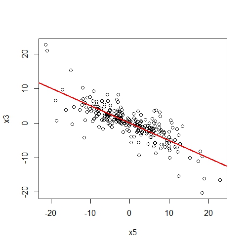
One might be interested in the partial effects of one variable on another given covariates in the SEM. The function partial.resid returns a data.frame of the partial residuals of y ~ x and plots the partial effect (if plotit = T).
# Load model package
library(nlme)

# Load data from Shipley (2013)
data(shipley2013)

# Create list of structured equations
shipley2013.modlist = list(

  lme(x2~x1, random = ~x1 | species, data = shipley2013),

  lme(x3~x2, random = ~x2 | species, data = shipley2013),

  lme(x4~x2, random = ~x2 | species, data = shipley2013),

  lme(x5~x3+x4, random = ~x3+x4 | species, data = shipley2013)

  )

# Get partial residuals of x3 on x5 conditional on x4
resids.df = partial.resid(x5 ~ x3, shipley2013.modlist, list(lmeControl(opt = "optim")))
###Get R2 for individual models
Return R2 and AIC values for component models in the SEM.
sem.model.fits(shipley2009.modlist)

#      Class   Family     Link  Marginal Conditional       AIC
#        lme gaussian identity 0.4864825   0.6990231 9166.9738
#        lme gaussian identity 0.4095855   0.9838829 4694.9821
#        lme gaussian identity 0.1079098   0.8366353 7611.3338
#   glmerMod binomial    logit 0.5589201   0.6291994  261.0824
###Return model predictions
Generate model predictions from new data.
# Create new data for predictions
shipley2009.new = data.frame(

  lat = rnorm(length(shipley2009$lat), mean(shipley2009$lat, na.rm = T),
    sd(shipley2009$lat, na.rm = T)),

  DD = rnorm(length(shipley2009$DD), mean(shipley2009$DD, na.rm = T),
    sd(shipley2009$DD, na.rm = T)),

  Date = rnorm(length(shipley2009$Date), mean(shipley2009$Date, na.rm = T),
    sd(shipley2009$Date, na.rm = T)),

  Growth = rnorm(length(shipley2009$Growth), mean(shipley2009$Growth, na.rm = T),
    sd(shipley2009$Growth, na.rm = T))

)

# Generate predictions
head(sem.predict(shipley2009.modlist, shipley2009.new))

#      lat       DD     Date   Growth   DD.fit Date.fit Growth.fit Live.fit
# 63.74900 156.6662 118.6954 50.95160 143.3918 120.3736   46.48266 5.497643
# 55.72110 134.5989 136.9055 51.32790 150.0989 131.3554   51.95870 5.628542
# 46.47976 151.3796 136.1517 61.89734 157.8198 123.0045   51.73203 9.305165
# 47.13647 133.6134 140.5558 50.41360 157.2712 131.8458   53.05642 5.310499
# 63.57681 161.3186 117.1850 50.50880 143.5357 118.0584   46.02848 5.343615
# 47.56635 137.4427 119.1214 49.35723 156.9120 129.9401   46.61076 4.943035

