This is a page to document some additional methods and techniques implemented in KataGo, such as some things not in (the latest version of) the arXiv paper, or that were invented or implemented or discovered by KataGo later, or that were drawn from other research or literature but not documented elsewhere in KataGo's paper or materials.
- Training on Multiple Board Sizes via Masking
- Fixup Initialization
- Shaped Dirichlet Noise
- Root Policy Softmax Temperature
- Policy Surprise Weighting
- Subtree Value Bias Correction
- Dynamic Variance-Scaled cPUCT
- Short-term Value and Score Targets
- Uncertainty-Weighted MCTS Playouts
- Nested Bottleneck Residual Nets
- Auxiliary Soft Policy Target
- Fixed Variance Initialization and One Batch Norm
- Optimistic Policy
(This method has been used in KataGo through all of its runs. It was presented in an early draft of its paper but was cut later for length limitations).
KataGo was possibly the first superhuman selfplay learning Go bot capable of playing on a wide range of board sizes using the same neural net. It trains the same neural net on all board sizes from 9x9 to 19x19 and reaches superhuman levels on all of them together. Although actual machine learning applications are often more flexible, in many deep learning literature tutorials and real ML training pipelines, it's common to require or to preprocess all inputs to be the same size. However, with the right method, it's straightforward to train a neural net that can handle inputs of variable sizes, even within a single batch.
The method consists of two parts. First, designing the neural net to not intrinsically require a certain size of board. Second, a masking trick that allows mixing multiple board sizes into the same batch during both training and inference, working around the fact that tensors in ML libraries and for GPUs have to be rectangular.
The first part is easier than one might expect. For example, convolution is a local operation that transforms values based only on their neighbors, so a convolutional layer can be applied to any size of input. Many common pooling layers and normalization layers are also size-independent. This means that almost all of a standard residual convolutional net can be applied identically regardless of whether the input is 9x9, or 19x19, or 32x32, or 57x193. The only tricky part sometimes is the output head. In much of the literature, you find that the output head is a set of fully-connected layers mapping C (channels) * H (height) * W (width) values to some final output(s). Such a head has weight dimensions that depend on H and W, so is not size-independent. However, it's not hard to construct alternate heads that are. For example, global average pooling the C * H * W channels down to just a fixed C channels before applying a fully-connected head. Or perhaps having a fixed C' different channels that are allowed to attend to spatial subregions of the C * H * W values, where attention weights are computed via convolutions. Or, depending on the application, perhaps the output head can simply be itself convolutional. KataGo uses a mix of these approaches variously for the policy and value heads and auxiliary heads.
With the net not hardcoded to any specific size, the second part is how to perform mixed-size batched training so that the learned weights are effective when applied to different sizes. For this, one can mix sizes into the same batch using a masking trick:
- Size the input tensor to the size of the largest input in that batch.
- Zero-pad each entry in the batch independently to fill out the excess space.
- Keep a 0-1 mask indicating which parts of the tensor are "real" space, rather than excess space, and apply the mask after each operation that would make the excess space nonzero.
- Additionally, if the net contains operations like channelwise average pooling or other things that depend on the spatial size, use a divisor based on the true spatial size, rather than the tensor size, so that the zeros in the excess space do not dilute the average. Whenever a convolution "peers over the edge" of its input, it will see only zeros, exactly the same as it would see with a zero-padding convolution if the tensor were properly sized to that entry. After operations like convolution, the padding space may no longer be all zero because the convolution will introduce nonzero values into the excess space. This can be solved simply by masking those entries back to 0, as illustrated below. Most nets add various kinds of scaling or normalization or bias layers between convolutional layers, and the masking can simply be included with that operation (fusing it into the same GPU kernel, if performance is desired), making it very, very cheap.
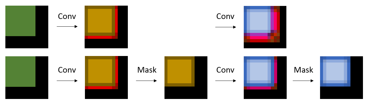 |
| Convolution produces values within oversized tensor area. Top: The next convolution corrupts the final blue square. Bottom: Masking ensures a final result independent of tensor size. |
The result of the above is that KataGo is able to train a single net on many board sizes simultaneously, generalizing across all of them. Although KataGo's recent 2020 run ("g170") only trained on sizes from 7x7 to 19x19, it appears to extrapolate quite effectively to larger boards, playing at a high level on board sizes in the 20s and 30s with no additional training. This demonstrates that the net has to some degree learned general rules for how size scaling should affect its predictions. Mixed-size training is also not particularly expensive. At least in early training up to human pro level, KataGo seems to learn at least equally fast and perhaps slightly faster than training on 19x19 alone. This is likely due to massive knowledge transfer between sizes, and because playing smaller boards with lower branching factors and game length might give faster feedback, which speeds up learning on larger boards. Outside of Go and board games, the suitability of this method may of course greatly depend on the application. For example, downsampling to make input sizes match might be more suitable than directly mixing sizes via the above method for an image processing application where different-sized images have intrinsically different levels of detail resolution, since variable resolution means the low-level task differs. In contrast, in Go, the local tactics always behave the same way per "pixel" of the board. Using the above method might also require some care in the construction of the final output head(s) depending on the task. But regardless, size-independent net architectures and mixing sizes via masking seem like useful tricks to have in one's toolbox.
(This method was used starting in "g170", KataGo's January 2020 to June 2020 run).
This method is NOT used any more in KataGo, see the Fixed Variance Initialization and One Batch Norm section below.
KataGo has been successfully training without batch normalization or any other normalization layers by using Fixup Initialization, a simple new technique published in ICLR 2019: https://arxiv.org/abs/1901.09321 (Zhang, Dauphin, and Ma, ICLR 2019).
KataGo's implementation of Fixup was fairly straightforward, with a minor adjustment due to using preactivation residual blocks. Within each residual block we:
-
Replace both of the batch-norm layers with just plain channelwise additive bias layers, initialized to 0.
-
Insert one channelwise multiplicative scaling layer, just before the final convolution, initialized to 1.
-
Initialize the first convolution weights of the block using the normal "He" initialization, except multiplied by
1/sqrt(total number of residual blocks). -
Initialize the second convolution weights of the block to 0.
And lastly, KataGo added a gradient clip. It appears that early in training when the net is still mostly random, rarely KataGo's training will experience batches causing very large gradient steps just due to the nature of the training data and high early learning rate. By forcibly scaling down scaling large activations, batch norm was preventing blowup. However, a gradient clip set at roughly a small constant factor larger than normal early-training gradients appeared to be just as effective. This only affected early training - past that, the gradient is almost never large enough to even come close to the clip limit.
Unlike what the authors of Fixup needed for their experiments, KataGo needed no additional regularization to reproduce and even surpass the quality of the original training.
Dropping batch normalization has resulted in some very nice advantages:
-
Much better performance on the training GPU. Batch norm is surprisingly expensive during gradient updates, removing it sped up training by something like 1.6x or 1.8x. This is not that important overall given that selfplay is most of the cost, but is still nice.
-
Simple logic for the neural net in different contexts. There is no longer a need to behave differently in training versus inference.
-
Because there is no longer cross-sample dependence in a batch or overt batch-size-dependence, easy to write things like multi-GPU training that splits apart batches while achieving mathematically identical results, or to vary the batch size without as much tricky hyperparameter tuning.
-
Avoidance of a few suspected problems caused by batch norm itself. Leela Chess Zero in an older run found an explicit problem caused by batch normalization where due to the rarity of activation of certain channels (but nonetheless highly-important rare activations, apparently used in situations where a pawn is about to promote), batch norm's per-batch normalization was not represented well by the inference-time scaling. Although KataGo did not test in enough detail to be sure, anecdotally KataGo experienced a few similar problems regarding Japanese vs Chinese rules when evaluating rare "seki" positions, which improved in runs without batch norm.
(This method was used starting in "g170", KataGo's January 2020 to June 2020 run).
Although this method is used in KataGo, due to heavy limits on testing resources, it has not been validated as a measurable improvement with controlled runs. The evidence for it should be considered merely suggestive, so this section is just here to describe the idea and intuition. However, to the extent that Dirichlet noise is useful, this method seems to have a much greater-than-baseline chance of noising true blind-spot moves the vast majority of the time, and therefore is included in KataGo's recent runs.
To give some background: to help unexpected new good moves to have a chance of being explored, AlphaZero-style self-play training replaces 25% of the root policy prior mass with Dirichlet-distributed noise, with Dirichlet alpha parameter of 0.03 per move. KataGo uses a "total alpha" of 10.83 = 361 * 0.03 divided across legal moves, so that the Dirichlet alpha parameter for each legal move on the empty 19x19 board matches that of AlphaZero's. Since the sum of the alphas is 10.83, interpretively, this can be loosely thought of as selecting "about 10.83" legal moves at random with replacement and assigning about 25% / 10 = 2.5% policy prior to each one (specifically, via a Polya's urn process). The Dirichlet alpha scales the likelihood of selection, so when alpha is spread uniformly, each legal move is equally likely to be selected.
When examining positions manually, one finds that the vast majority of the time, even "blind spot" moves with very low policy priors have higher policy priors than most legal moves on the board. Even if the absolute prior is low, like only 0.05%, this is often still much higher than most obviously bad moves (moves on the first line, moves that add stones within one's own completely alive territory, moves that threaten absolutely nothing, etc.).
Therefore, KataGo tries to shape the Dirichlet noise to increase the likelihood that such moves are noised and explored. Using an arbitrary formula based on the log of the policy prior (see the code for details), KataGo distributes only half of the total alpha uniformly, and concentrates the other half of the alpha on the smaller subset of moves that still have a policy much higher in logits than most other legal moves.
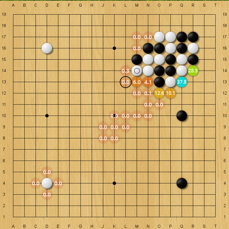 |
| Blind spot for an older 40-block KataGo net, policy prior. The correct move L13 has only an 0.008% policy prior on this evaluation, but is still higher than almost all arbitrary moves on the board. (Every unlabeled move is lower in policy prior than it). |
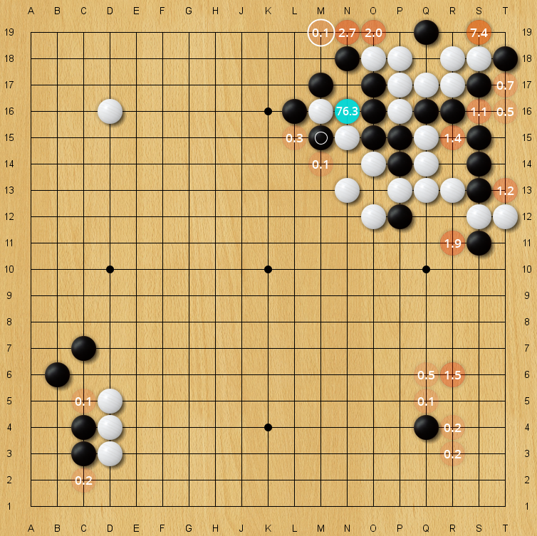 |
| Blind spot for an older 40-block KataGo net, policy prior. The correct move M19 has only an 0.11% policy prior on this evaluation, but is still higher than almost all arbitrary moves on the board. (Every unlabeled move is lower in policy prior than it). |
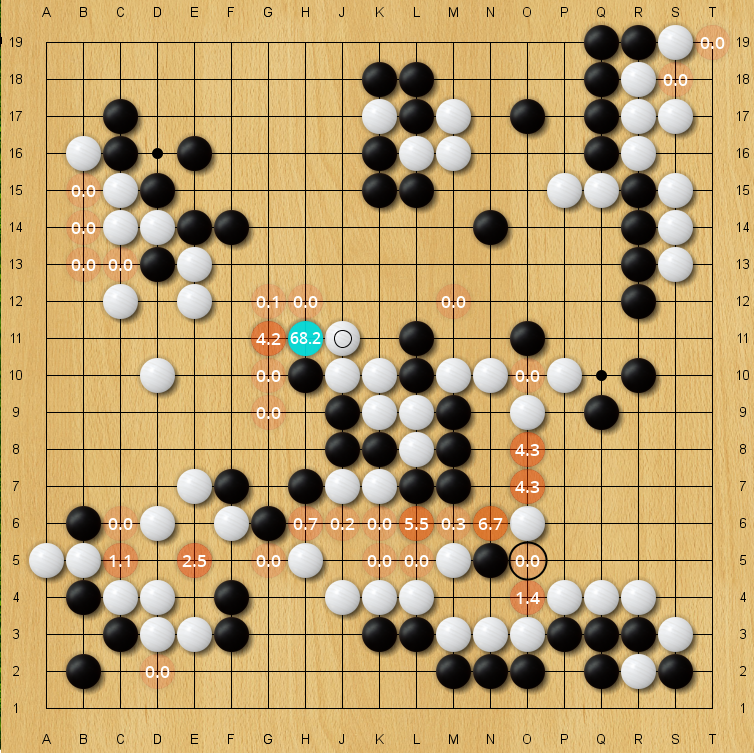 |
| Blind spot for an older 40-block KataGo net, policy prior. The correct move O5 has only an 0.03% policy prior on this evaluation, but is still higher than almost all arbitrary moves on the board. (Every unlabeled move is lower in policy prior than it). |
Note that the ability of KataGo to discriminate between moves even in such extreme realms of unlikelihood is improved by policy target pruning as described in KataGo's paper. Without policy target pruning, moves with policy prior like 0.008% might be obscured by the haze of probability mass assigned uniformly to all moves in the neural net's attempt to predict the background of noise playouts, which in turn would probably make this technique of shaped Dirichlet noise less effective.
(This method was used starting in "g170", KataGo's January 2020 to June 2020 run).
KataGo uses the same technique as SAI used to stabilize some of its early runs and improve exploration and counter the above dynamic - which is to use a softmax temperature slightly above 1 applied to the policy prior before adding Dirichlet noise or using the policy prior in the search. In KataGo's g170 run, this temperature was 1.25 for the early game, decaying exponentially to 1.1 for the rest of the game with a halflife in turns of the board dimensions (e.g. 9 or 19). This scaling is only applied at the root node.
When viewed in logit space, this temperature scaling is equivalent to scaling all logits towards 0 by a factor of 1.1, or 1.25, and requires the MCTS search to actively counteract this force to maintain policy sharpness. This ensures that moves will not decay in policy prior if the MCTS search finds them to have a utility comparable to the best alternative moves, with no evidence that the move is worse.
The motivation for this approach is to observe that in the baseline AlphaZero algorithm, due to the dynamics of the PUCT formula, there is a slight tendency for the most preferred move in a position to become even more strongly preferred, even when that move is valued equally to its alternatives. If one runs an MCTS search with a given policy prior, where the utility value of the top move is fixed and equal to that of the best alternative moves, due to the +1 in the denominator of the formula and the discretization of the search, the MCTS visit distribution will generally be sharper than the prior, despite zero evidence having been obtained by the search that the move is better than its alternatives.
Additionally, in early opening positions in games like Go, the policy sometimes becomes opinionated a little too quickly between nearly-equal moves, limiting exploration. It may be that the search disfavors a given move due to consistently undervaluing a tactic, so the entire training window fills with data that reinforces that undervaluation, leading the policy for the move to converge to nearly zero. (Dirichlet noise helps, but alone doesn't prevent this.)
Therefore, having policy softmax temperature act as a restoring force pushing the policy back towards uniform among moves that are extremely similarly-valued should be useful for improving exploration.
(This method was used starting in "g170", KataGo's January 2020 to June 2020 run).
KataGo overweights the frequency of training samples where the policy training target was "highly surprising" relative to the policy prior. Conveniently, in the process of generating self-play training data, we can know exactly how surprising one of the most recent neural nets would have found that data since we can just look at the policy prior on the root node. This method is one of the larger improvements in KataGo's training between its g170 run and earlier runs.
In detail: normally, KataGo would record each position that was given a "full" search instead of a "fast" search (see "Playout Cap Randomization" here KataGo's paper for understanding "full" vs "fast" searches) with a "frequency weight" of 1 in the training data, i.e. writing it into the training data once. With Policy Surprise Weighting, instead, among all full-searched moves in the game, KataGo redistributes their frequency weights so that about half of the total frequency weight is assigned uniformly, giving a baseline frequency weight of 0.5, and the other half of the frequency weight is distributed proportionally to the KL-divergence from the policy prior to the policy training target for that move. Then, each position is written down in the training data floor(frequency_weight) many times, as well as an additional time with a probability of frequency_weight - floor(frequency_weight). This results in "surprising" positions being written down much more often.
In KataGo, the method used is not like importance sampling where the position is seen more often but the gradient of the sample is scaled down proportionally to the increased frequency, to avoid bias. We simply sample the position more frequently, using full weight for the sample. The purpose of the policy is simply to suggest moves for MCTS exploration, and unlike a predictive classifier or stochastically sampling a distribution or other similar methods where having an unbiased output is good, biasing rare good moves upward and having them learned a bit more quickly seems fairly innocuous (and in the theoretical limit of optimal play, any policy distribution supported on the set of optimal moves is equally optimal).
Some additional minor notes:
- Due to an arbitrary implementation choice, KataGo uses the noised softmaxed root policy prior, rather than the raw prior. Possibly using the raw prior would be very slightly better, although it might require changing other hyperparameters.
- The frequency weight of a full search is actually not always 1. It might be lower near the end of the game due to KataGo's "soft resignation" scheme, where instead of resigning a self-play training game, KataGo conducts faster and lower-weighted searches to finish the game past the point where AlphaZero or Leela Zero would have resigned, to avoid introducing pathological biases in the training data.
- KataGo allows "fast" searches to get a nonzero frequency weight if despite the lower number of playouts, the fast search still found a result that was very surprising, using a somewhat arbitrary and not-particularly-carefully-tuned cutoff threshold for the required KL-divergence to be included.
- Additionally, in KataGo we also add a small weight for surprising utility value samples, rather than just surprising policy samples, but this is much more experimental and unproven.
(This method was discovered a few months after the end of KataGo's "g170" run).
As of late 2020, KataGo has tentatively found a heuristic method to improve MCTS search evaluation accuracy in Go. Fascinatingly, it is of the same flavor as older methods like RAVE in classic MCTS bots, or the history heuristic in alpha-beta bots, or pattern-based logic in Go bots between 2010 and 2015. Many of these methods have fallen out of use in post-AlphaZero MCTS due to being no longer helpful and often harmful. Intuitively this is due to the fact that compared to a neural net that actually "understands" the board position, such blind heuristics are vastly inferior. Possibly the reason why this method could still have value is because rather than attempting to provide an absolute estimate of utility value, it instead focuses on online-learning of some correlated errors, or bias in the value from the neural net at nodes relative to values from deeper search in the node's subtree - i.e. attempting to bootstrap a correction rather than coming up with the value afresh.
While similar things may have been invented and published elsewhere, as of late 2020, I am personally unaware of anything quite like this that has been successful in post-AlphaZero MCTS bots. This method adjusts only the utility estimates of MCTS search tree nodes. Exploration and the PUCT formula remain unchanged, except for taking the new utility values as input. The method is as follows:
Firstly, we write the relationship that defines the MCTS utility of a search tree node in a mathematically equivalent but slightly different form than usually presented. Normally in AlphaZero-style MCTS, the MCTS utility estimate for a node during the search is the running average of the raw heuristic utility estimates from the neural net or other evaluation function, which here we call "NodeUtility", averaged over all playouts that passed through that node. Here, instead of expressing it as a running statistical average of the playouts that have been sent through that node, we define it as a recurrence based on its children. We define the MCTS utility of each search node n in terms of the raw heuristic utility estimate of that node and of the utility of its children c by:
For a node that has at least one child, we also track the observed error of the neural net's raw utility prediction relative to its subtree, which we presume is probably a more accurate estimate due to the deeper search:
In normal MCTS search, we would have NNUtility = NodeUtility (i.e. the neural net's raw value estimate of node are what get averaged in the running statistics), but as we will see below, for this method we distinguish the two.
We bucket all nodes in the search tree using the following combination as the key:
- The player who made the last move.
- The location of the last move (treating "pass" as a location).
- The location of the move before last move (treating "pass" as a location).
- If the last move was not a pass, the 5x5 pattern (Black, White, Empty, Off-board) surrounding the last move, as well as which stones in that pattern were in atari.
- If the previous move made a move illegal due to ko ban, the location of that ko ban.
For each bucket B, we define its weighted average observed bias:
Then, instead of defining NodeUtility to be equal to the neural net's utility prediction on that node (as in normal MCTS), we define NodeUtility to be a "bias-corrected" value that adjusts the raw neural net evaluation:
Every time a playout finishes, while walking back up the tree, in the process of recomputing each node's MCTS utility to take into account the result, for that node's bucket, we also recompute the bucket's ObsBias based on the updated ObsError for that node. Then, we also immediately retrieve that ObsBias value to update this node's NodeUtility. This also applies to leaf nodes that are not game-terminal positions - when a node is created at the end of a search tree branch, it immediately retrieves the ObsBias for the bucket it belongs to (although, of course, since the node has no children yet with which to compute its own error, it does not affect the bucket's ObsBias yet).
The rest of MCTS proceeds exactly as normal, except using these bias-adjusted NodeUtility values instead of the original NNUtility values (and which, unlike the NNUtility values, can "retroactively" update later as the bucket values change), and the resulting MCTSUtility values that result from averaging them.
In KataGo, currently we only retrieve a new ObsBias value for a node from its bucket as we walk through that node following a playout. Nodes in other parts of the tree may grow slightly stale as the observed bias for their bucket changes but will update the next time they are visited. KataGo also has a bit of handling that carries over part of the weight of buckets during search tree reuse between turns when some parts of the tree are lost but others remain. KataGo currently finds lambda = 0.35 and alpha = 0.8 to be a very significant improvement over normal MCTS, ranging from 30 to 60 Elo.
The intuition behind all of this is to correct for persistent biases in the neural net's evaluation regarding certain sequences of play in an online fashion. For example, the neural net might persistently judge a particular sequence of moves as initially promising, but will realize upon deeper search that actually the result is bad. This tactic may be explored in many different branches of the search tree, over and over, each time being judged promising, explored, and giving a bad result. Or, the reverse may happen, with a repeated tactic always coming out better than the net initially predicts. By bucketing nodes by the local pattern, once one of the explorations of a tactic has gone deep enough to realize a more accurate evaluation, subsequent explorations of that tactic elsewhere will use neural net evaluations that are bias-corrected proportional to the weighted average observed error between the neural net at the start of the tactic and the subtrees of the search that explore the tactic.
By only averaging errors in a bucket rather than absolute utilities, we continue to leverage the neural net's overall ability to predict the utility far more accurately than any crude heuristic. Each different place in a search tree that a tactic is visited, changes may have occurred elsewhere on the board that significantly affect the overall expected utility in a way that only a sophisticated net can judge in absolute terms. However, the error in the neural net's evaluation of this local tactic relative to that overall level may still be consistent. This is possibly the reason why at least in early testing, this method still seems beneficial, whereas other methods that deal with absolute utilities, like RAVE, are not so useful in modern bots.
(This method was first experimented with in KataGo in early 2021, and released in June 2021 with v1.9.0).
This method can be motivated and explained by a simple observation. Consider the PUCT formula that controls exploitation versus exploration in modern AlphaZero-style MCTS:
Suppose for a given game/subgame/situation/tactic the value of the cPUCT coefficient is k. Then, consider a game/subgame/situation/tactic that is identical except all the differences between all the Q values at every node are doubled (e.g. the differences between the winrates of moves and the results of playouts are doubled). In this new game, the optimal cPUCT coefficient is now 2k because a coefficient of 2k is what is needed to exactly replicate the original search behavior, given that the differences in Q are all twice as large as before.
In other words, all else equal, if the scale of utility differences between moves changes, the optimal cPUCT coefficient should change proportionally. Since the scale of utility differences varies across games and situations within a game, using a constant value for cPUCT for the entire game does not make sense.
So, as of mid 2021, KataGo now:
- Keeps track of the empirical variance of the utility of the playouts for each search node in the tree, mixing in a small prior to get a reasonable variance estimate for nodes with too few playouts.
- At every node, scales the cPUCT for choosing which children of that node to explore by roughly sqrt(utility variance).
So KataGo now uses cPUCT that dynamically adjusts proportionally with the empirical scale of variations in utility. Another intuition for why this should give better results:
- If the utility of playouts is varying wildly, you should explore more and not overly exploit the first high-value move you see, since wild variation means other moves have more chance to be better too, even if they initially look worse.
- If the utility is varying only a tiny bit and estimates are very stable, you should focus in and optimize more precisely between these fine differences, rather than continuing to invest in spreading playouts over a wide range of moves that consistently perform worse than the best move.
Combined with the uncertainty weighting method below, KataGo as of version 1.9.0 seems to be about 75 Elo stronger than the preceding release, and about 50 Elo stronger than the preceding release if the cPUCT for the preceding release is optimally tuned (with the latest networks, apparently about 25 Elo could be gained by tuning a better constant cPUCT).
(This method has been used since since "g170", KataGo's January 2020 to June 2020 run).
KataGo trains the neural net to predict several auxiliary value targets, which exponentially average future MCTS values:
(1-lambda) sum_{t' >= t} MCTS_value(t') lambda^(t'-t)
There are three targets, each using a different lambda, so that the mean time horizon is roughly the next 6 turns, 16 turns, and 50 turns into the future on a 19x19 board, and correspondingly shorter for smaller boards in proportion to the board area. There are also auxiliary score heads and targets analogous to the value heads. The various loss weights used on these auxiliary value and score heads have varied over different training runs, but generally, neural nets seem to train slightly faster and achieve slightly better value and score loss on the main head that tries to predict the final game result (corresponding to lambda -> 1.0) by simply decreasing the loss weight a little on the main head and adding these additional heads. Presumably, these additional heads provide lower-variance feedback on the value of a position, in a classic bias-variance tradeoff.
This has not been fully re-tested with recent nets in a controlled way, but a partial test was done in late 2022, shown here. Below is an old plot of the value loss on a fixed self-play dataset extracted from KataGo's training data, testing from-scratch training of a net using a legacy value loss weighting that weighted long-term values heavily, compared to from-scratch training of a net equal-weighting them. This should be considered more illustrative of the magnitude of the possible effect from such weightings and not a particularly careful or rigorous test of the benefit of this method, especially since it doesn't show the effect of overall loss weight changes or have a control that exclusively uses only the final-game-outcome target.
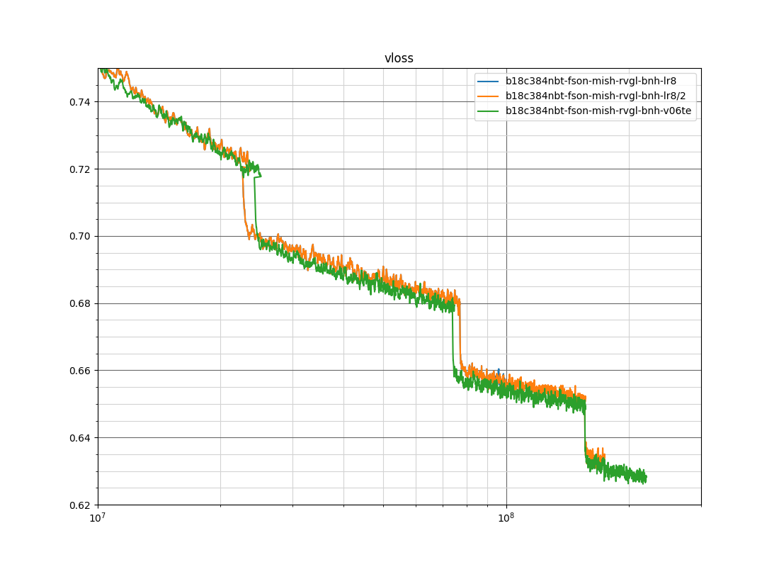 |
| Value loss in predicting the final game outcome in early b18c384nbt neural net training with different weightings on predicting different exponential average time horizons [final outcome, 50 turns, 16 turns, 6 turns]. ORANGE: an older and legacy loss weight configuration [1.0,0.458,0.458.0.125]. GREEN: equal-weighted [0.6, 0.6, 0.6, 0.6]. Y axis is the unweighted loss of the value head that predicts the final outcome, X axis is the number of training steps in samples. |
Arguably the more important benefit of these auxiliary targets is not on improving the value prediction (although it is nice and free to the degree that it exists!), but rather that having short-term predictions enables further methods below, see Uncertainty-Weighted MCTS Playouts and Optimistic Policy.
(This method was first experimented with in KataGo in early 2021, and released in June 2021 with v1.9.0).
KataGo now weights different MCTS playouts according to the "confidence" of the neural net's utility estimates for that playout, downweighting playouts where the neural net reports that its estimate is likely to have high error, and upweighting those that the neural net is confident in.
Specifically on any given turn t in the game, we train the neural net to predict the short-term error between its current output and the values from MCTS from the training data that are treated as the ground truth:
- Predict the squared difference between
stop_gradient(neural net's current short-term value prediction)and(1-lambda) sum_{t' >= t} MCTS_value(t') lambda^(t'-t) - Predict the squared difference between
stop_gradient(neural net's current short-term score prediction)and(1-lambda) sum_{t' >= t} MCTS_score(t') lambda^(t'-t)
Where MCTS_value(t') and MCTS_score(t') are the root value and score from MCTS recorded for turn t' in the training data, and lambda ~= 5/6 (on 19x19 boards) is an arbitrary coefficient for computing an exponential weighted average over the subsequent turns. Smaller boards adjust lambda so that the average amount into the future is smaller roughly proportional to the board area. The stop-gradient is so that the neural net attempts to adjust the error prediction heads to match this squared difference, but do not attempt to adjust the value and score prediction heads to make the squared difference closer to the error prediction head's output. For the loss function, we also just use squared error, i.e. the loss is fourth-degree in the underlying values. (Actually, we use Huber loss, which is basically just squared error but avoiding extreme outliers).
Basically, the neural net not only produces a winrate and score, but also an estimate of how uncertain or inaccurate those winrates and scores are relative to what a search would conclude a few turns later. We then simply downweight playouts roughly proportionally to the neural net's reported uncertainty, so that uncertain playouts count as a "fraction of a playout" for the purposes of computing the MCTS average values and for driving the PUCT exploration formula, and highly certain playouts count as "more than one playout" for these. We add a small minimum baseline uncertainty so as to cap the maximum weight that one single playout can provide.
From manual observations by hand this uncertainty prediction behaves almost exactly as one would hope. It is low in calm positions and smooth positions where there are lots of moves that are all reasonable choices with similar values, such as in many openings. It spikes up when fights break out and in the middle of unresolved tactics, then falls again when the tactic resolves.
Combined with the dynamic cPUCT method above, KataGo as of 1.9.0 release seems to be about 75 Elo stronger than the preceding release, and about 50 Elo stronger than the preceding release if the cPUCT for the preceding release is optimally tuned (with the latest networks, apparently about 25 Elo could be gained by tuning a better constant cPUCT).
(This method was first experimented with in KataGo at the end of 2022, and became part of main-run nets in March 2023 with v1.13.0).
This method was inspired by the appendix of the Gumbel Muzero paper (Danhelka et al, ICLR 2022). Many thanks to the authors of that work, particularly Julian Schrittwieser for raising it to attention.
In that paper's appendix, the authors note an improved architecture for convolutional neural nets in Go, which is to use a bottleneck residual net. However, they use a slightly longer bottleneck than the normal one you see in the literature elsewhere.
A basic (pre-activation) residual block looks like the following:
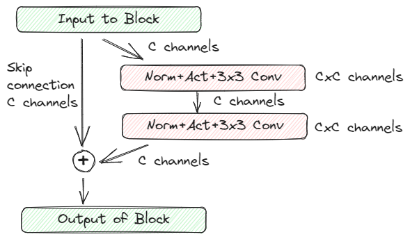
A bottleneck residual block attempts to be computationally cheaper by reducing the dimension via 1x1 convolutions, before doing the 3x3 convolution which is where the expensive bulk of the computation happens. Hoping that the computation is more efficient as a composition of lower-rank operations, this can allow you to stack more total blocks or increase the number of channels C a little.
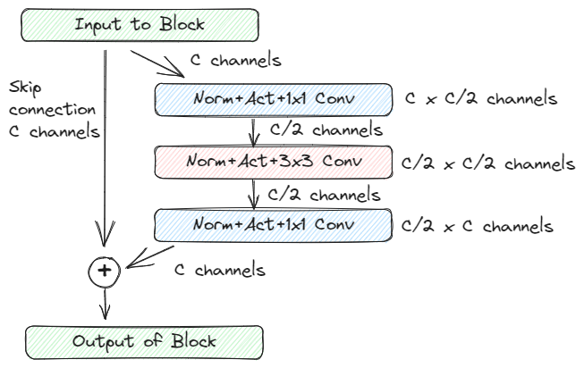
However, in early development KataGo already tested this and found it was substantially worse than normal residual blocks, holding total compute cost constant. The interesting observation in the Gumbel Muzero paper appendix is that the following block (handwaving away differences of preactivation vs postactivation) is better than normal residual blocks:
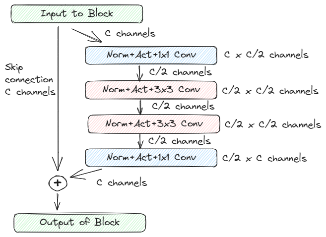
In retrospect, this makes sense. 1x1 convolutions are still fairly expensive, and only doing one 3x3 convolution at reduced dimension per pair of 1x1 convolutions doesn't pay back the cost. But doing two of them does pay back the cost! KataGo found that in its particular use case, in fact going to three or four was slightly better, further reducing the relative overhead of the 1x1 convs:
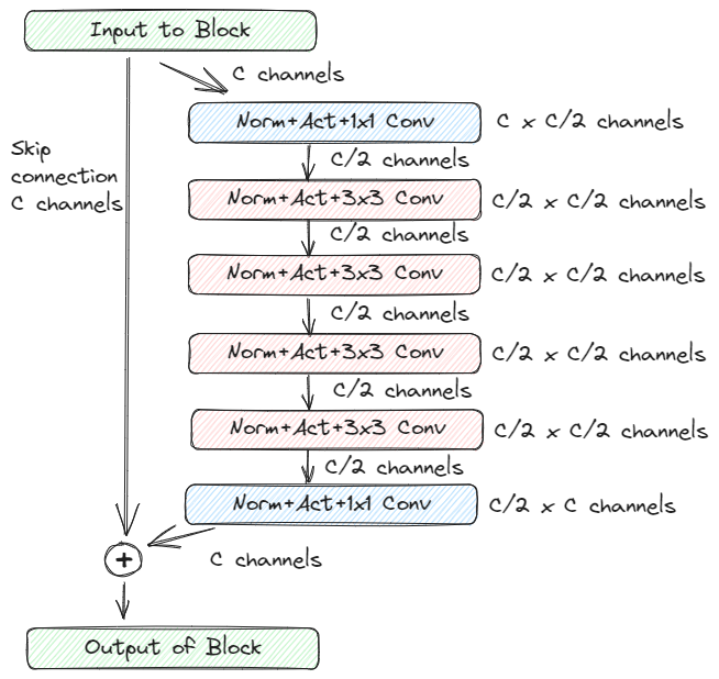
Once we're at four 3x3 convs though, it's pretty natural to pair them up into their own residual blocks by adding skip connections, to improve optimization. This results in the final improved block architecture that KataGo uses, as of mid 2023:
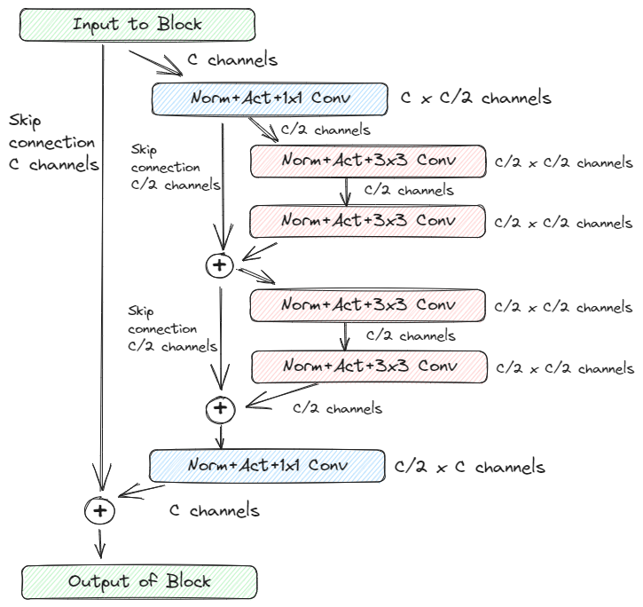
This is one of a few improvements to KataGo's neural net architecture and training in 2022-2023, which together along with some other tuning resulted in a new "b18c384" net, of comparable speed to the older "b40c256" nets, sometimes slightly faster, yet only barely weaker-per-evaluation than the old twice-as-heavy "b60c320" nets.
(This method was first experimented with in KataGo at the end of 2022, and became part of main-run nets in March 2023 with v1.12.0).
This method was suggested for KataGo by an excellent user "lionfenfen" based on their independent research. Many thanks to them! The exact parameters and weighting KataGo uses has changed since the initial suggestion, but either way the method appears to greatly improves the speed of learning of the policy.
The method is simple:
Add an auxiliary policy head that attempts to predict the policy target raised to power of (1/T) for some moderately large temperature T (and re-normalized to sum to 1).
Simply adding this auxiliary "soft" policy target also improves the learning of the original policy head, at least for KataGo. At first, this might seem a bit surprising. Why would predicting the the exact same data under just a simple transformation improve things?
As intuition, consider a policy target like:
60% A
36% B
3% C
1% D
<0.1% on a few other moves.
Under cross entropy loss, the policy will be heavily incentivized to learn correctly-weighted predictions for A and B. However, there will be little pressure to the policy to get the weight of C and D correct vs each other and vs other moves. If the policy assigns 1% for C, 2% for D, and puts a whole 3% on some other move entirely, the loss is only barely greater than if it predicts 3% and 1% accurately for C and D.
The softer policy^(1/T) might look like:
30% A
26% B
14% C
11% D
<6% on a few other moves
Predicting this well requires recognizing that MCTS liked C and D more than other moves, and also predicting roughly by how much. Thanks to policy target pruning as described in KataGo's paper, a lot of the low-mass moves in KataGo's policy target are not purely noise from Dirichlet noise, but rather contain meaningful information about how much MCTS liked that move. Presumably, learning to discriminate this much richer target beyond just usually predicting the best 1-2 moves helps the neural net form better internal features, improving the learning.
KataGo currently uses T = 4 and also weights the soft policy target nominally 8 times more than the normal policy target. The 8x nominal weight compensates for the fact that after reasonably optimized, the soft policy provides much smaller gradients on average.
This is one of a few improvements to KataGo's neural net architecture and training in 2022-2023, which together along with some other tuning resulted in a new "b18c384" net, of comparable speed to the older "b40c256" nets, sometimes slightly faster, yet only barely weaker-per-evaluation than the old twice-as-heavy "b60c320" nets.
(This method was first experimented with in KataGo at the end of 2022, and became part of main-run nets in March 2023 with v1.12.0).
This method replaces Fixup Initialization above. This development is also partially thanks to users "Medwin" and "lionfenfen" for motivating KataGo to re-test batch-norm and related normalization methods. This method seems to be better than FixUp, and capture some more of the benefit of BatchNorm while still avoiding the headaches of tuning Batch Renorm appropriately or having a major train/inference discrepancy in the neural net.
This is one of a few improvements to KataGo's neural net architecture and training in 2022-2023, which together along with some other tuning resulted in a new much stronger-per-compute "b18c384" net, although this particular improvement is probably more of a fixing of a historical suboptimal choice rather than being fundamentally much better than the best alternative state-of-the-art methods.
Firstly, we initialize the neural net in a manner different than Fixup:
In every place in the neural net where a batch normalization layer would normally be inserted, we add a simple scalar multiplication by a fixed layer-specific constant K. The way we determine K is to idealize every convolution-activation layer pair in the net as outputting random values with the same variance as they receive as input, to assume that the variance of a sum is the sum of its variances, and to assume the input of the entire net is variance 1. Then, K is the unique value such that the output of the normalization layer is variance 1.
For example, here is how the nested bottleneck residual block from above would be normalized:
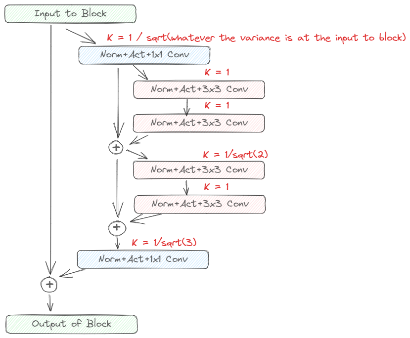
The variance accumulates to be larger than 1 due to the summations with skip connections, but every normalization layer chooses the scaling that resets the variance following it to back 1. By itself, this appears to work at least as well in KataGo as Fixup, but is a more general rule, so can be applied to more complex architectures that Fixup doesn't describe how to handle, such as this nested residual block.
Secondly:
- We add one batch norm layer to the neural net, at the end of the trunk of blocks, just before the point where the policy head, value head, etc. all attach.
- We attach a second independently-learning copy of all heads with exactly the same loss functions to the trunk without the batch norm layer.
- The first set of heads that goes through the batch norm layer is given most of the loss weight (currently 80%).
- The second set of heads that skips the batch norm layer is given less loss weight (currently 20%), and are the heads that are used at inference time.
This seems to recover most (but not all) of the optimization benefit of batch norm. The idea is that the first set of heads is mostly the one driving optimization during training since it has most of the loss weight. Since it goes through a batch norm layer, this removes most of the incentive throughout the rest of the net for weights to adjust their overall magnitudes, similar to as if there were batch norm layers throughout the net. The second set of heads learns to make optimal predictions given the same features without normalization, so it can be directly used at inference time without having to track moving averages of batch normalization layers and creating an annoying train/inference difference in the net.
(This method was developed through 2022 and the first half of 2023, and became part of main-run nets in June 2023 with v1.13.0).
Thanks to Reid McIlroy-Young, Craig Falls, and a few unnamed others for some of the discussions and inspiration leading to this method. Many thanks also to various members of the Computer Go discord channel for helping test this. This method builds off of the short-term targets in Short-term Value and Score Targets the short-term error predictions of those targets in Uncertainty-Weighted MCTS Playouts.
We train an additional policy head alongside the normal policy on the exact same policy target as the normal policy head, except that we softly restrict to data samples where the player to move got a surprisingly higher value or score in the shortterm outcome in the selfplay data than the neural net expected.
Specifically we weight the policy target by:
clamp(0.0, 1.0, sigmoid((z_value-1.5)*3) + sigmoid((z_score-1.5)*3))
where:
z_value = (shortterm_value_outcome - stop_grad(shortterm_value_pred)) / stop_grad(sqrt(shortterm_value_squared_error_pred + epsilon))
and analogously for z_score. The shortterm_value_outcome is the same roughly-6-turn (on 19x19, shorter on smaller boards) exponentially weighted short-term future MCTS value described in earlier sections, and shortterm_value_pred is the output of the auxiliary value head that predicts it and shortterm_value_squared_error_pred is the output of the auxiliary head that predicts the expected squared error. epsilon is a small constant to avoid division by values too close to zero. The two stop_grads ensure that error on the optimistic policy doesn't flow backwards and cause the net to reassess what it thought the value or expected value error was.
The specific formulas above are somewhat arbitrary, and the 'best' formula is unknown. The intent is to train an optimistic policy head that predicts the policy conditioned on the current player's MCTS being able to find a variation that turns out to be much better than expected. This formula gives full weight or nearly full weight to training samples where such a surprise happens, and small but nonzero weight in all other cases, which regularizes the policy to reduce to just the normal policy in cases when no surprise is possible.
Then, during MCTS at test-time, we use the optimistic policy for both sides during the search. In KataGo, this appears to be worth something like 40 to 90 Elo, depending on other settings. The exact mechanism for why this is good is unknown, but here are some possible hypotheses (which are the same intuitions that motivated trying this method to begin with and probably are ways to phrase different aspects of a similar underlying idea):
-
Often, an unexpectedly good result is due to MCTS finding a surprising good tactic that the raw model didn't spot. The optimistic policy is more likely to suggest lines of play that may lead to such moves, so that MCTS can more thoroughly check whether there is such a tactic or not. Similar to multi-armed bandit methods that explore optimistically based on a confidence bound rather than only picking the highest average.
-
Ever since the dawn of computer Chess programs back in the mid-1900s, the horizon effect has plagued computer game AIs, where the losing player will interpose many useless or even self-harming "timesuji" or horizon-delaying moves as the game starts to swing against them. Sticking their head in the sand trying to delay the inevitable. Modern AlphaZero-based programs are no exception, and the policy will in fact learn such moves in self-play. The optimistic policy may weigh these moves less since pointless delaying moves will occur much more when the player is imminently about to lose, rather than when they are imminently about to unexpectedly get a good result.
-
Human players familiar with solving Chess puzzles, or tsumego in Go, will understand this concept intuitively - the "toughest resistance" that you need to consider for the opponent resisting you is often NOT the line the opponent should play in a real game. Rather, the opponent should often back down after the very first move and give you what you want, to cut their losses. But the concession line is not the line you need to evaluate to determine whether the tactic works or not; you need to evaluate the line where both players resist and escalate, heedless of the fact that if such a line were actually played in real life (rather than only being simulated within the search), the opponent's willingness to escalate right back would be Bayesian evidence that maybe they can refute you after all. The optimistic policy may be better at solving these critical lines since on each player's turn it optimistically conditions on that player being the imminent winner and suggests moves appropriate to that optimism, rather than being inclined to already concede within the search to a tactic before proving that it works.
Although it would not be hard to change later, as of June 2023, the optimistic policy is not used during self-play since it is not clear what happens if this pretty substantial way of biasing the policy is fed back on itself - whether it is sound or whether it may lead to some convergence issues down the line.