-
Notifications
You must be signed in to change notification settings - Fork 1
/
README.qmd
380 lines (290 loc) · 14.1 KB
/
README.qmd
1
2
3
4
5
6
7
8
9
10
11
12
13
14
15
16
17
18
19
20
21
22
23
24
25
26
27
28
29
30
31
32
33
34
35
36
37
38
39
40
41
42
43
44
45
46
47
48
49
50
51
52
53
54
55
56
57
58
59
60
61
62
63
64
65
66
67
68
69
70
71
72
73
74
75
76
77
78
79
80
81
82
83
84
85
86
87
88
89
90
91
92
93
94
95
96
97
98
99
100
101
102
103
104
105
106
107
108
109
110
111
112
113
114
115
116
117
118
119
120
121
122
123
124
125
126
127
128
129
130
131
132
133
134
135
136
137
138
139
140
141
142
143
144
145
146
147
148
149
150
151
152
153
154
155
156
157
158
159
160
161
162
163
164
165
166
167
168
169
170
171
172
173
174
175
176
177
178
179
180
181
182
183
184
185
186
187
188
189
190
191
192
193
194
195
196
197
198
199
200
201
202
203
204
205
206
207
208
209
210
211
212
213
214
215
216
217
218
219
220
221
222
223
224
225
226
227
228
229
230
231
232
233
234
235
236
237
238
239
240
241
242
243
244
245
246
247
248
249
250
251
252
253
254
255
256
257
258
259
260
261
262
263
264
265
266
267
268
269
270
271
272
273
274
275
276
277
278
279
280
281
282
283
284
285
286
287
288
289
290
291
292
293
294
295
296
297
298
299
300
301
302
303
304
305
306
307
308
309
310
311
312
313
314
315
316
317
318
319
320
321
322
323
324
325
326
327
328
329
330
331
332
333
334
335
336
337
338
339
340
341
342
343
344
345
346
347
348
349
350
351
352
353
354
355
356
357
358
359
360
361
362
363
364
365
366
367
368
369
370
371
372
373
374
375
376
377
378
379
380
---
format: gfm
bibliography: vignettes/references.bib
execute:
message: false
warning: false
# knitr:
# opts_chunk:
# fig.path: "man/figures/README-"
eval: false
default-image-extension: ""
---
# spanishoddata: Get Spanish Origin-Destination Data <a href="https://rOpenSpain.github.io/spanishoddata/"><img src="man/figures/logo.png" align="right" width="200" alt="spanishoddata website" /></a>
<!-- badges: start -->
[](https://www.repostatus.org/#active)
[](https://lifecycle.r-lib.org/articles/stages.html#stable){target="_blank"} [](https://CRAN.R-project.org/package=spanishoddata){target="_blank"}
[](https://CRAN.R-project.org/package=spanishoddata){target="_blank"}
[](https://CRAN.R-project.org/package=spanishoddata){target="_blank"}
[](https://github.com/rOpenSpain/spanishoddata/actions/workflows/R-CMD-check.yaml)
[](https://doi.org/10.32614/CRAN.package.spanishoddata)
[](https://doi.org/10.5281/zenodo.14516104)
<!-- 10.5281/zenodo.14516104 -->
<!-- badges: end -->
**spanishoddata** is an R package that provides functions for downloading and formatting Spanish open mobility data released by the Ministry of Transport and Sustainable Mobility of Spain [@mitma_mobility_2024_v8].
It supports the two versions of the Spanish mobility data that consists of origin-destination matrices and some additional data sets. [The first version](https://www.transportes.gob.es/ministerio/proyectos-singulares/estudios-de-movilidad-con-big-data/estudios-de-movilidad-anteriores/covid-19/opendata-movilidad) covers data from 2020 and 2021, including the period of the COVID-19 pandemic. [The second version](https://www.transportes.gob.es/ministerio/proyectos-singulares/estudios-de-movilidad-con-big-data/opendata-movilidad) contains data from January 2022 onwards and is regularly updated. Both versions of the data primarily consist of mobile phone positioning data, and include matrices for overnight stays, individual movements, and trips of Spanish residents at different geographical levels. See the [package website](https://rOpenSpain.github.io/spanishoddata/) and vignettes for [v1](https://rOpenSpain.github.io/spanishoddata/articles/v1-2020-2021-mitma-data-codebook) and [v2](https://rOpenSpain.github.io/spanishoddata/articles/v2-2022-onwards-mitma-data-codebook) data for more details.
**spanishoddata** is designed to save time by providing the data in analysis-ready formats. Automating the process of downloading, cleaning, and importing the data can also reduce the risk of errors in the laborious process of data preparation. It also reduces computational resources by using computationally efficient packages behind the scenes. To effectively work with multiple data files, it’s recommended you set up a data directory where the package can search for the data and download only the files that are not already present.
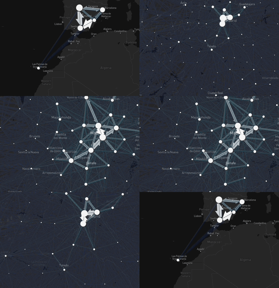
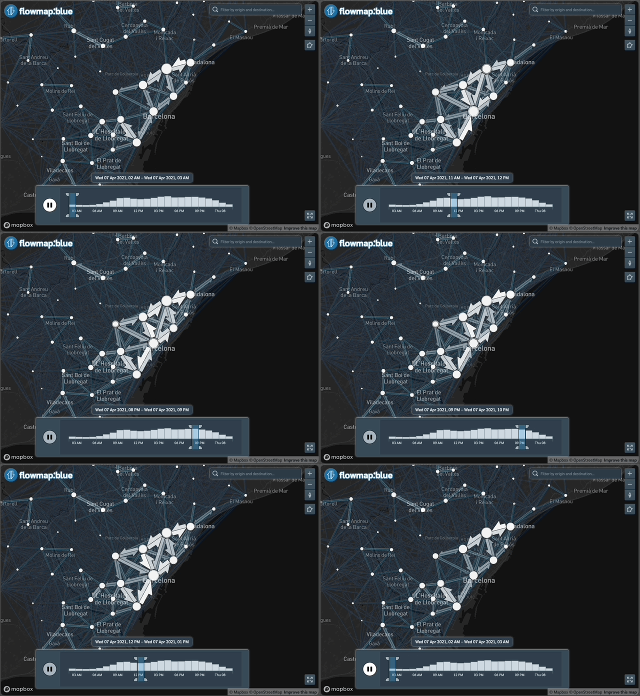
# Examples of available data
{#fig-barcelona-flows}
To create static maps like that see our vignette [here](https://ropenspain.github.io/spanishoddata/articles/flowmaps-static.html).
---
{#fig-spain-flows}
{#fig-spain-flows}
To create interactive maps see our vignette [here](https://ropenspain.github.io/spanishoddata/articles/flowmaps-interactive.html).
{{< include inst/vignette-include/install-package.qmd >}}
Load it as follows:
```{r}
library(spanishoddata)
```
{{< include inst/vignette-include/setup-data-directory.qmd >}}
{{< include inst/vignette-include/overall-approach.qmd >}}
{#fig-overall-flow width="78%"}
# Showcase
To run the code in this README we will use the following setup:
```{r}
#| label: pkgs
library(tidyverse)
theme_set(theme_minimal())
sf::sf_use_s2(FALSE)
```
```{r}
#| include: false
remotes::install_github("r-tmap/tmap")
```
Get metadata for the datasets as follows (we are using version 2 data covering years 2022 and onwards):
```{r}
#| label: metadata
metadata <- spod_available_data(ver = 2) # for version 2 of the data
metadata
```
```
# A tibble: 9,442 × 6
target_url pub_ts file_extension data_ym data_ymd
<chr> <dttm> <chr> <date> <date>
1 https://movilidad-o… 2024-07-30 10:54:08 gz NA 2022-10-23
2 https://movilidad-o… 2024-07-30 10:51:07 gz NA 2022-10-22
3 https://movilidad-o… 2024-07-30 10:47:52 gz NA 2022-10-20
4 https://movilidad-o… 2024-07-30 10:14:55 gz NA 2022-10-18
5 https://movilidad-o… 2024-07-30 10:11:58 gz NA 2022-10-17
6 https://movilidad-o… 2024-07-30 10:09:03 gz NA 2022-10-12
7 https://movilidad-o… 2024-07-30 10:05:57 gz NA 2022-10-07
8 https://movilidad-o… 2024-07-30 10:02:12 gz NA 2022-08-07
9 https://movilidad-o… 2024-07-30 09:58:34 gz NA 2022-08-06
10 https://movilidad-o… 2024-07-30 09:54:30 gz NA 2022-08-05
# ℹ 9,432 more rows
# ℹ 1 more variable: local_path <chr>
```
## Zones
Zones can be downloaded as follows:
```{r}
#| label: distritos
distritos <- spod_get_zones("distritos", ver = 2)
distritos_wgs84 <- distritos |>
sf::st_simplify(dTolerance = 200) |>
sf::st_transform(4326)
plot(sf::st_geometry(distritos_wgs84))
```

## OD data
```{r}
od_db <- spod_get(
type = "origin-destination",
zones = "districts",
dates = c(start = "2024-03-01", end = "2024-03-07")
)
class(od_db)
```
```
[1] "tbl_duckdb_connection" "tbl_dbi" "tbl_sql"
[4] "tbl_lazy" "tbl"
```
```{r}
colnames(od_db)
```
```
[1] "full_date" "time_slot"
[3] "id_origin" "id_destination"
[5] "distance" "activity_origin"
[7] "activity_destination" "study_possible_origin"
[9] "study_possible_destination" "residence_province_ine_code"
[11] "residence_province" "income"
[13] "age" "sex"
[15] "n_trips" "trips_total_length_km"
[17] "year" "month"
[19] "day"
```
The result is an R database interface object (`tbl_dbi`) that can be used with dplyr functions and SQL queries 'lazily', meaning that the data is not loaded into memory until it is needed.
Let's do an aggregation to find the total number trips per hour over the 7 days:
```{r}
#| label: trips-per-hour
n_per_hour <- od_db |>
group_by(date, time_slot) |>
summarise(n = n(), Trips = sum(n_trips)) |>
collect() |>
mutate(Time = lubridate::ymd_h(paste0(date, time_slot, sep = " "))) |>
mutate(Day = lubridate::wday(Time, label = TRUE))
n_per_hour |>
ggplot(aes(x = Time, y = Trips)) +
geom_line(aes(colour = Day)) +
labs(title = "Number of trips per hour over 7 days")
```

The figure above summarises 925,874,012 trips over the 7 days associated with 135,866,524 records.
## `spanishoddata` advantage over accessing the data yourself
As we demonstrated above, you can perform very quick analysis using just a few lines of code.
To highlight the benefits of the package, here is how you would do this manually:
- download the [xml](https://movilidad-opendata.mitma.es/RSS.xml) file with the download links
- parse this xml to extract the download links
- write a script to download the files and locate them on disk in a logical manner
- figure out the data structure of the downloaded files, read the codebook
- translate the data (columns and values) into English, if you are not familiar with Spanish
- write a script to load the data into the database or figure out a way to claculate summaries on multiple files
- and much more...
We did all of that for you and present you with a few simple functions that get you straight to the data in one line of code, and you are ready to run any analysis on it.
# Desire lines
We'll use the same input data to pick-out the most important flows in Spain, with a focus on longer trips for visualisation:
```{r}
od_national_aggregated <- od_db |>
group_by(id_origin, id_destination) |>
summarise(Trips = sum(n_trips), .groups = "drop") |>
filter(Trips > 500) |>
collect() |>
arrange(desc(Trips))
od_national_aggregated
```
```
# A tibble: 96,404 × 3
id_origin id_destination Trips
<fct> <fct> <dbl>
1 2807908 2807908 2441404.
2 0801910 0801910 2112188.
3 0801902 0801902 2013618.
4 2807916 2807916 1821504.
5 2807911 2807911 1785981.
6 04902 04902 1690606.
7 2807913 2807913 1504484.
8 2807910 2807910 1299586.
9 0704004 0704004 1287122.
10 28106 28106 1286058.
# ℹ 96,394 more rows
```
The results show that the largest flows are intra-zonal.
Let's keep only the inter-zonal flows:
```{r}
od_national_interzonal <- od_national_aggregated |>
filter(id_origin != id_destination)
```
We can convert these to geographic data with the {od} package [@lovelace_od_2024]:
```{r}
#| label: desire-lines
od_national_sf <- od::od_to_sf(
od_national_interzonal,
z = distritos_wgs84
)
distritos_wgs84 |>
ggplot() +
geom_sf(aes(fill = population)) +
geom_sf(data = spData::world, fill = NA, colour = "black") +
geom_sf(aes(size = Trips), colour = "blue", data = od_national_sf) +
coord_sf(xlim = c(-10, 5), ylim = c(35, 45)) +
theme_void()
```

Let's focus on trips in and around a particular area (Salamanca):
```{r}
#| label: salamanca-zones
salamanca_zones <- zonebuilder::zb_zone("Salamanca")
distritos_salamanca <- distritos_wgs84[salamanca_zones, ]
plot(distritos_salamanca)
```

We will use this information to subset the rows, to capture all movement within the study area:
```{r}
#| label: salamanca
ids_salamanca <- distritos_salamanca$id
od_salamanca <- od_national_sf |>
filter(id_origin %in% ids_salamanca) |>
filter(id_destination %in% ids_salamanca) |>
arrange(Trips)
```
Let's plot the results:
```{r}
#| label: salamanca-plot
od_salamanca_sf <- od::od_to_sf(
od_salamanca,
z = distritos_salamanca
)
ggplot() +
geom_sf(fill = "grey", data = distritos_salamanca) +
geom_sf(aes(colour = Trips), size = 1, data = od_salamanca_sf) +
scale_colour_viridis_c() +
theme_void()
```

# Further information
For more information on the package, see:
- The [pkgdown site](https://rOpenSpain.github.io/spanishoddata/)
- [Functions reference](https://rOpenSpain.github.io/spanishoddata/reference/index.html)
- [v1 data (2020-2021) codebook](https://rOpenSpain.github.io/spanishoddata/articles/v1-2020-2021-mitma-data-codebook.html)
- [v2 data (2022 onwards) codebook (work in progress)](https://rOpenSpain.github.io/spanishoddata/articles/v2-2022-onwards-mitma-data-codebook.html)
- [Download and convert data](https://rOpenSpain.github.io/spanishoddata/articles/convert.html)
- The [OD disaggregation vignette](https://rOpenSpain.github.io/spanishoddata/articles/disaggregation.html) showcases flows disaggregation
- [Making static flowmaps](https://rOpenSpain.github.io/spanishoddata/articles/flowmaps-static.html) vignette shows how to create flowmaps using the data acquired with `{spanishoddata}`
- [Making interactive flowmaps](https://rOpenSpain.github.io/spanishoddata/articles/flowmaps-interactive.html) shows how to create an interactive flowmap using the data acquired with `{spanishoddata}`
- [Quickly getting daily aggregated 2022+ data at municipality level](https://ropenspain.github.io/spanishoddata/articles/quick-get.html)
```{r}
#| label: repo-setup
#| eval: false
#| echo: false
# Create data-raw and data folders
usethis::use_data_raw()
usethis::use_description()
usethis::use_r("get.R")
usethis::use_package("glue")
usethis::use_package("xml2")
# ‘fs’ ‘lubridate’ ‘stringr’
usethis::use_package("fs")
usethis::use_package("lubridate")
usethis::use_package("stringr")
devtools::check()
# Set-up pkgdown + ci
usethis::use_pkgdown()
usethis::use_github_action("pkgdown")
# Setup gh pages:
usethis::use_github_pages()
# Auto-style with styler
styler::style_pkg()
usethis::use_tidy_description()
```
## Citation
```{r}
#| eval: true
#| echo: false
#| results: 'asis'
print(citation("spanishoddata"), bibtex = FALSE)
```
BibTeX:
```
```{r}
#| eval: true
#| echo: false
#| results: 'asis'
toBibtex(citation("spanishoddata"))
```
```
# References
<!-- metadata for better search engine indexing -->
<!-- should be picked up by pkgdown -->
<!-- update metadata before release with -->
<!-- cffr::cff_write() -->
<!-- codemetar::write_codemeta(write_minimeta = T) -->
```{r}
#| eval: true
#| include: false
is_html <- knitr::is_html_output()
```
```{r results="asis", eval = !is_html, include = !is_html, include = FALSE}
glue::glue('<script type="application/ld+json">
{glue::glue_collapse(readLines("inst/schemaorg.json"), sep = "\n")}
</script>')
```