Using Gaia data to make some plots for open clusters and analysing them.
Star cluster plots are scraped from the VizieR database with Selenium, as implemented in trawl_vizier.py. The trawler file takes around half an hour to run - querying and capturing the raw CMDs from VizieR's plotter. These images undergo some basic transforms (a mirror flip and a rotation) for a better understanding in the fix_images.py file. The 1229 cluster plots are now analysed and here we select 10 plots for further analysis. These clusters selected are IC 4651, IC 4756, NGC 752, NGC 1664, NGC 2281, NGC 2287, NGC 2527, NGC 6281, NGC 6405, NGC 6475. If you already have selected clusters for analysis, proceed to the next step rather than perform these again.
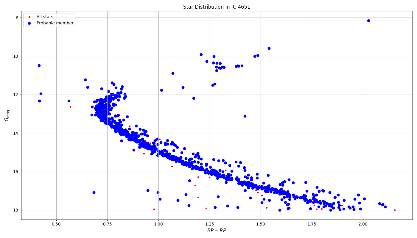
The data related to these clusters are taken from the WEBDA database and added to the select.json file. The star data is downloaded into csv files by the get_multiple_clusters.py file. Here, plots of the raw data are also made. We can arbitrarily split the points which correspond to binaries and single stars already. The generate_radec.py file lists out celestial coordinates for all star targets in the data and saves them in a file. This is done to query information about the stars by using the corresponding the celestial coordinates.
Properties of the cluster in select.json:
For every cluster in the file, under its name, there are multiple listed properties needed for the calculations. These properties are described as:
- "isochrone": The age of the parsec isochrone to be downloaded from CMD's database
- "distance": The distance of the cluster from Earth, in parsecs
- "g_corr": A correction added to the magnitude axis to get the isochrone to fit
- "b_corr": A correction added to the color axis to get the isochrone to fit
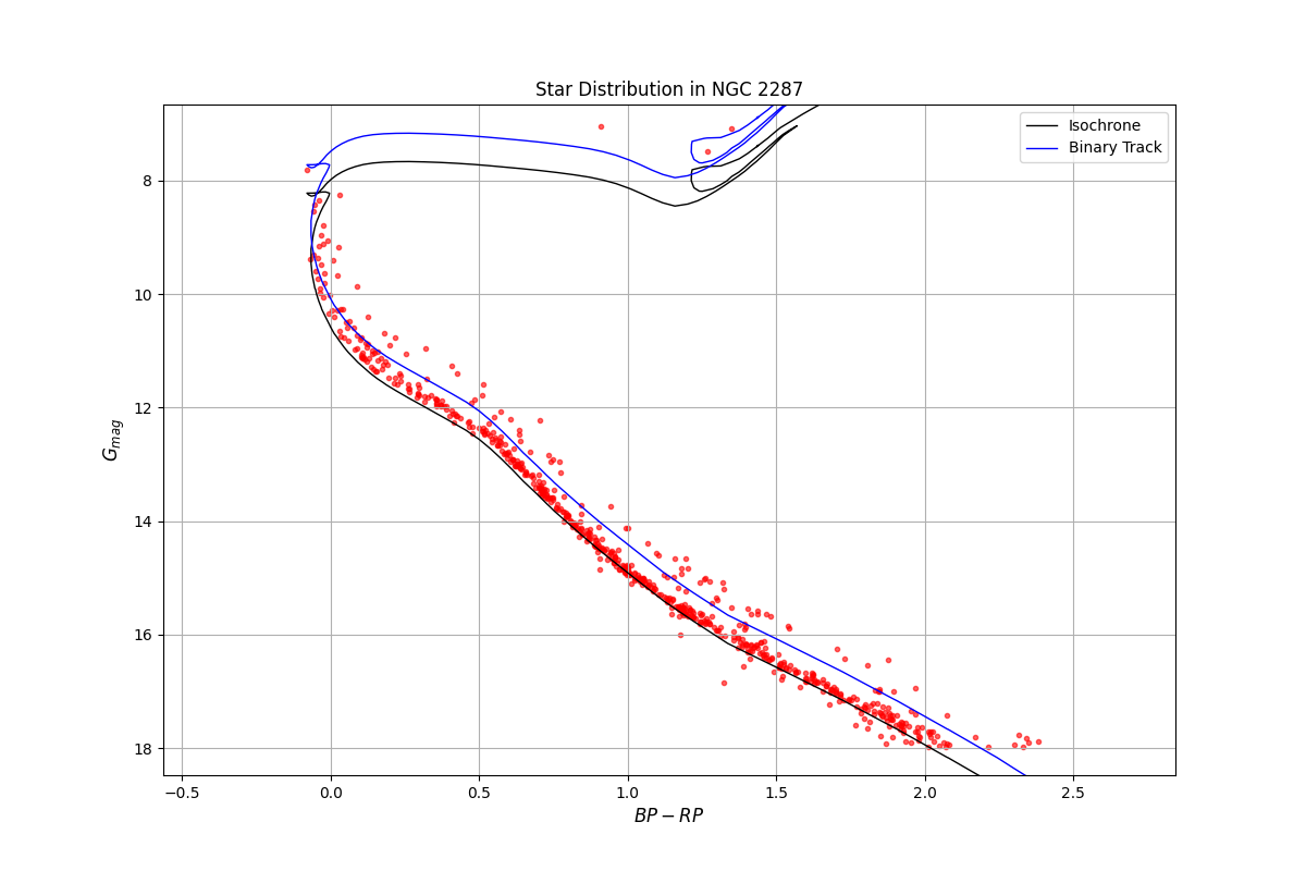
- "diff_corr": The difference between the isochrone and the curve splitting the binary track
- "metallicity": The metallicity value for the stars in the cluster
- "centerRA": The right ascension of the center of the cluster
- "centerDE": The declination of the center of the cluster
- "cluster_r": The radius of the cluster in arcminutes in the sky
- "central_r": The radius of the core of the cluster in arcminutes
- "mass_fn": The list of coefficients of the polynomial for mass calculation
- "AG": The estimated extinction coefficient for the cluster
- "E_BP-RP": The estimated E_BP-RP for the cluster
The data from WEBDA is then also used to download parsec isochrones from the CMD database. The website is automated with Selenium again to fill in the form as in download_isochrones.py. The downloaded data is now processed in read_isochrones.py. It generates a fitted isochrone with the cluster plot. The toggling of the purpose of the read_isochrones.py file is done by passing command line arguments while executing the file. It has the method to separate the single and binary track. Passing the argument show with the file highlights individual points in the plot. Otherwise the file defaults to saving a new copy of the isochrone tracks. Passing cluster names additionally allows for overwriting the file where the binary track is saved. Additionally, all can be passed to select and rewrite binaries for all clusters. This will be triggered only if show is passed before.
center_clusters.py uses the mean shift algorithm as implemented by scikit-learn and determines the centers of the clusters. Then the astropy module is used to compute the radial distance between the targets and the cluster center. The radial distribution plot for the single and binary track is also generated by this file. mass_distr.py has code to fit a polynomial to find the mass function for each cluster. central_density.py is used to calculate the central density of the cluster by analysing its core.
The /report/ directory has the tex files and bib files used to generate the project report where a more detailed overview of the project is given. The BibTeX distribution is used for LaTeX.
- python 3.8.5
- astropy 4.2
- matplotlib 3.3.3
- numpy 1.19.4
- pandas 1.2.1
- scikit-learn 0.24.0
- mplcursors 0.4
- selenium 3.141.0