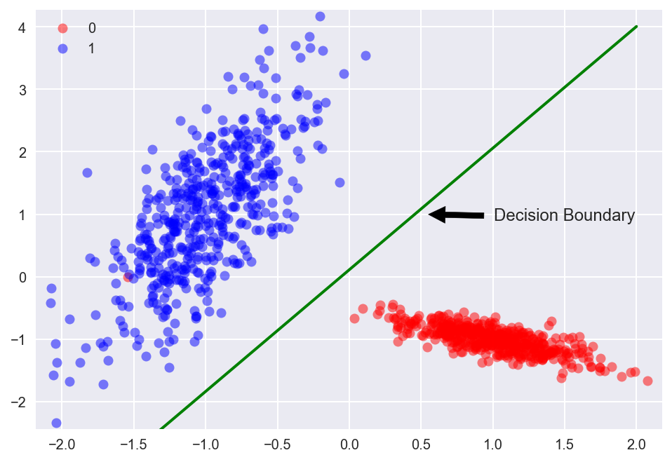
class based on petal_length and petal_width
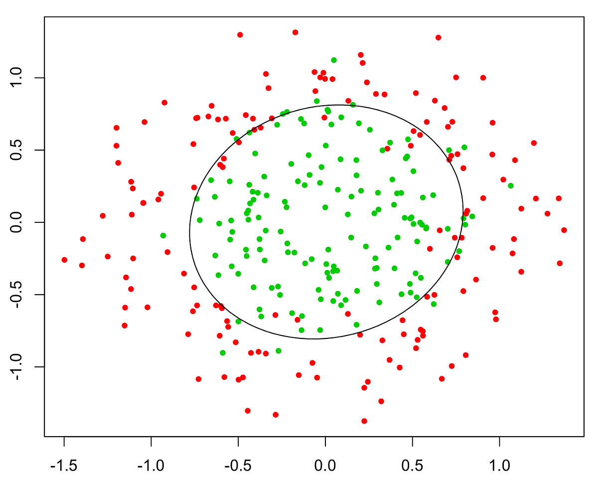
validity based on param_1 and param_2
28x28 pixel images.
28x28 pixel images.
Logistic regression is the appropriate regression analysis to conduct when the dependent variable is dichotomous (binary). Like all regression analyses, the logistic regression is a predictive analysis. Logistic regression is used to describe data and to explain the relationship between one dependent binary variable and one or more nominal, ordinal, interval or ratio-level independent variables.
Logistic Regression is used when the dependent variable (target) is categorical.
For example:
- To predict whether an email is spam (1) or (0).
- Whether online transaction is fraudulent (1) or not (0).
- Whether the tumor is malignant (1) or not (0).
In other words the dependant variable (output) for logistic regression model may be described as:
Training set is an input data where for every predefined set of features x we have a correct classification y.
m - number of training set examples.
For convenience of notation, define:
The equation that gets features and parameters as an input and predicts the value as an output (i.e. predict if the email is spam or not based on some email characteristics).
Where g() is a sigmoid function.
Now we my write down the hypothesis as follows:
Function that shows how accurate the predictions of the hypothesis are with current set of parameters.
Cost function may be simplified to the following one-liner:
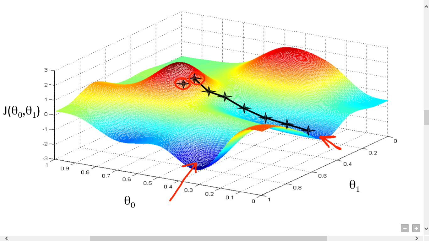
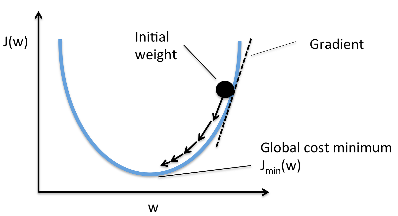
Gradient descent is an iterative optimization algorithm for finding the minimum of a cost function described above. To find a local minimum of a function using gradient descent, one takes steps proportional to the negative of the gradient (or approximate gradient) of the function at the current point.
Picture below illustrates the steps we take going down of the hill to find local minimum.
The direction of the step is defined by derivative of the cost function in current point.
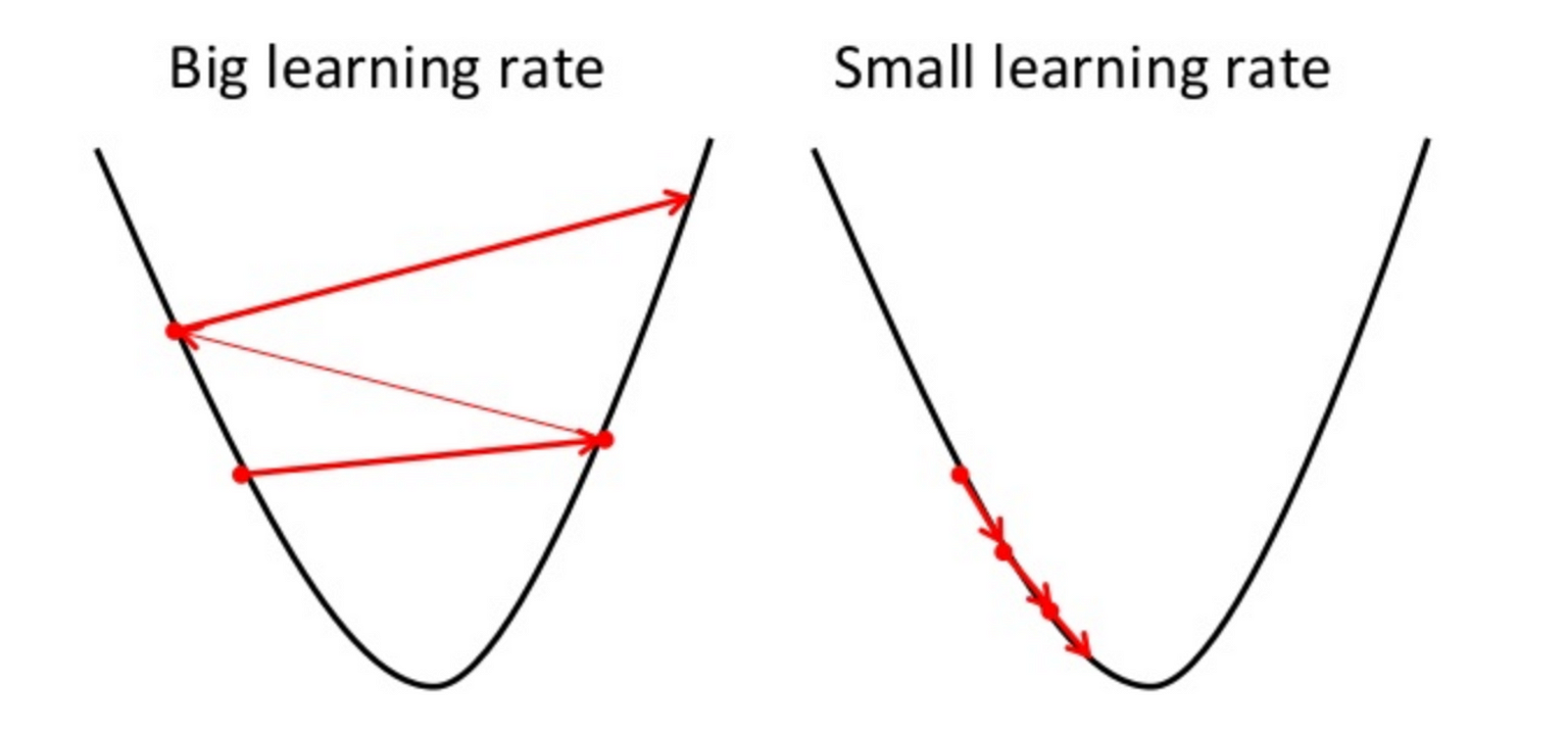
Once we decided what direction we need to go we need to decide what the size of the step we need to take.
We need to simultaneously update 


yi - output of ith training example
m - number of training examples
n - number of features
When we use term "batch" for gradient descent it means that each step of gradient descent uses all the training examples (as you might see from the formula above).
Very often we need to do not just binary (0/1) classification but rather multi-class ones, like:
- Weather: Sunny, Cloudy, Rain, Snow
- Email tagging: Work, Friends, Family
To handle these type of issues we may train a logistic regression classifier 
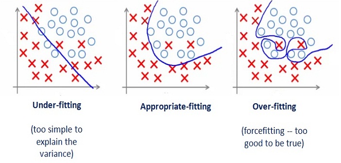
If we have too many features, the learned hypothesis may fit the training set very well:
But it may fail to generalize to new examples (let's say predict prices on new example of detecting if new messages are spam).
Here are couple of options that may be addressed:
- Reduce the number of features
- Manually select which features to keep
- Model selection algorithm
- Regularization
- Keep all the features, but reduce magnitude/values of model parameters (thetas).
- Works well when we have a lot of features, each of which contributes a bit to predicting y.
Regularization works by adding regularization parameter to the cost function:
In this case the gradient descent formula will look like the following:

