1. Start with MOVIS
In order to capture its full potential, we recommend using a Docker container of MOVIS.
Access MOVIS on this https://movis.mathematik.uni-marburg.de/ and start exploring your data! Depending on your internet connection, you might have difficulties uploading big data sets. To circumvent this, please use our Docker image.
This is the preferred method of running MOVIS. You should provide at least 6GB of memory to a docker instance. MOVIS container is hosted on DockerHub at https://hub.docker.com/r/aanzel/movis. To pull the docker container, enter the following sequence of commands into your terminal:
docker pull aanzel/movis:latest
docker run --publish 8501:8501 --detach --name movis aanzel/movis:latest
In order to access MOVIS, enter this URL http://localhost:8501/ into your internet browser of choice.
Caution! Use at your own risk!
You could also clone the GitHub repository, build a docker container yourself, and run it locally. This is not recommended as we might introduce unstable features that might not end in the next release of MOVIS. Below is a sequence of instructions to run the unstable version of MOVIS:
git clone https://github.com/AAnzel/MOVIS.git
cd MOVIS
docker build -t movis-local:unstable .
docker run --publish 8501:8501 --detach --name movis movis-local:unstable
You can start using the tool by opening a web browser and typing in http://localhost:8501/ as the address. If you run the docker container, you have to use the IP address or hostname instead of localhost.
Currently, MOVIS supports genomics, proteomics, metabolomics, transcriptomics, and physico-chemical time-series data sets. Multiple types and formats of data that MOVIS supports for each omic are presented below:
- Genomics:
- Archived FASTA files
- Archived BIN annotation files
- Archived KEGG annotation files
- Depth-of-coverage files
- Tabular file
- Proteomics:
- Archived FASTA files
- Tabular file
- Metabolomics
- Tabular file
- Transcriptomics
- Depth-of-coverage files
- One or many tabular files
- Physico-chemical
- Tabular file
Archived data sets are supported in the following formats: TARBZ2, TBZ2, TARGZ, TGZ, TAR, TARXZ, TXZ, ZIP. The size of the data set must be less than 200MB. This can be changed for the Docker version.
FASTA, BIN, KEGG, and Depth-of-coverage files must adhere to naming convection in order to be parsed correctly. In order to have temporality information, these files must be named using one of the following schemes:
- D03.{fa, gff, KOs.besthits, anything} for {FASTA, BIN, KEGG, Depth-of-coverage} file collected on the third day, or W03.{fa, gff, KOs.besthits, anything} for {FASTA, BIN, KEGG Depth-of-coverage} file collected on the third week. You will be given an option to select the start date.
-
2019-03-15.{fa, gff, KOs.besthits, anything} for {FASTA, BIN, KEGG, Depth-of-coverage} file collected on 15.03.2019. This is known as
ISO 8601standard format.
You should use either the first or the second option, mixing name options is not allowed.
File content of the archived data set must adhere to the following rules:
- FASTA: Sequences in a FASTA file can, but don't need to have a header.
- BIN: BIN annotation file content must contain lines with tab-separated information, and most importantly, the product information. One example is given below:
D01_contig_100340 Prodigal:2.6 CDS 1257 1856 . + 0 ID=A01_O1.2.4_PROKKA_56941;gene=srpR_2;inference=ab initio prediction:Prodigal:2.6,similar to AA sequence:UniProtKB:Q9R9T9;locus_tag=PROKKA_56941;product=HTH-type transcriptional regulator SrpR
-
KEGG: KEGG annotation file content must contain lines with tab-separated information according to this header
Gene ID maxScore hitNumber. One example is given below:
Gene	ID	maxScore	hitNumber
D01_L1.35_PROKKA_53162	KEGG:K04575	99.0	1
- Depth-of-coverage: Depth-of-coverage file content should contain two tab-separated columns. The first column should have the ID of the organism, and the second column should contain a number that depicts the depth-of-coverage value. One example is given below:
PROKKA_00001	5.31945
PROKKA_00006	6.19913
PROKKA_00032	7.86294
Tabular files are supported in CSV or TSV format and a maximum of 200MB in size. The size limit can be changed for the Docker version.
Tabular data sets must have one or two temporal columns named as one of the following: DateTime, Date, Time, Hour, Minute. If there are two columns, it is expected they have different names, and they will be merged by MOVIS into one column named DateTime.
If there are unknown values, MOVIS will remove all lines that contain those values. We intend to introduce data imputation to MOVIS in order to cover these types of data sets. Until then, if you want to work with data set that contain unknown values in some form, you should re-format them to your own liking.
In the case of transcriptomics data, users can upload multiple tabular data sets. However, each data set must have the same set of columns with exactly the same names. MOVIS concatenates these data sets into one unified data set with one new feature (column) named Type. This column contains names of all user-uploaded files. Multi-tabular functionality is provided to enable easier work with multiple biological replicate files at the same time, which is common when researching gene expression.
The sidebar holds navigation and general information about MOVIS. With the sidebar, you can easily navigate example pages and/or look for documentation, fill a bug report, or propose a new feature to be added to MOVIS. You can see the look of the sidebar below. The homepage contains more information about MOVIS and rudimentary instructions on how to use it. At the bottom of the homepage is a Changelog section with the history of changes to the tool. You can see the look of the homepage below.
The Example 1 page uses a data set from the following paper:
Herold, M., Martínez Arbas, S., Narayanasamy, S. et al. Integration of time-series meta-omics data reveals how microbial ecosystems respond to disturbance. Nat Commun 11, 5281(2020). https://doi.org/10.1038/s41467-020-19006-2.
The user is first presented with this information, along with a precise location on the map where the samples were collected (or processed). This data set contains genomics, metabolomics, proteomics, and physico-chemical data.
The Example 2 page uses a data set from the following paper: This data set comes from the following paper:
Merchel Piovesan Pereira, B., Wang, X., & Tagkopoulos, I. (2020). Short- and Long-Term Transcriptomic Responses of Escherichia coli to Biocides: a Systems Analysis. Applied and environmental microbiology, 86(14), e00708-20. https://doi.org/10.1128/AEM.00708-20.
As with the Example 1 page, a user is also presented with location information of data collection (processing). This data set contains transcriptomics data.
The Case study page is created using data from Example 1. It is constructed to showcase the power of MOVIS in exploring temporal multi-omics data sets. This page has multiple data sets preloaded/preselected so that a user can easily follow a case study story created for the original MOVIS manuscript.
After getting accustomed to MOVIS using the provided Example pages, users can upload their own data sets on the Upload page. A user can choose which kind of omics are of relevance and upload data sets for the selected options. When a user chooses a new omic, the main window is split to support the new choice. If MOVIS is used as a web service, then there is a capacity limit of 200MB per file. If you are running MOVIS docker container locally, there is no capacity limit. On top of the upload button, various supported formats are laid out.
Below are presented various screenshots of MOVIS. Each screenshot depicts one or more essential functionalities or showcases a different part of the tool that the user experiences.
The homepage. The default page is a welcome page that briefly describes the tool and provides a changelog.
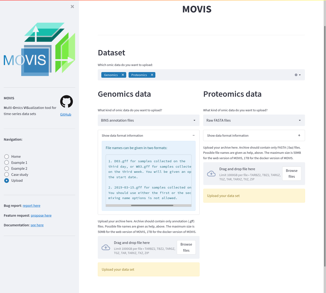
Screenshot of the upload functionality. Genomics and proteomics data are ready to be uploaded.
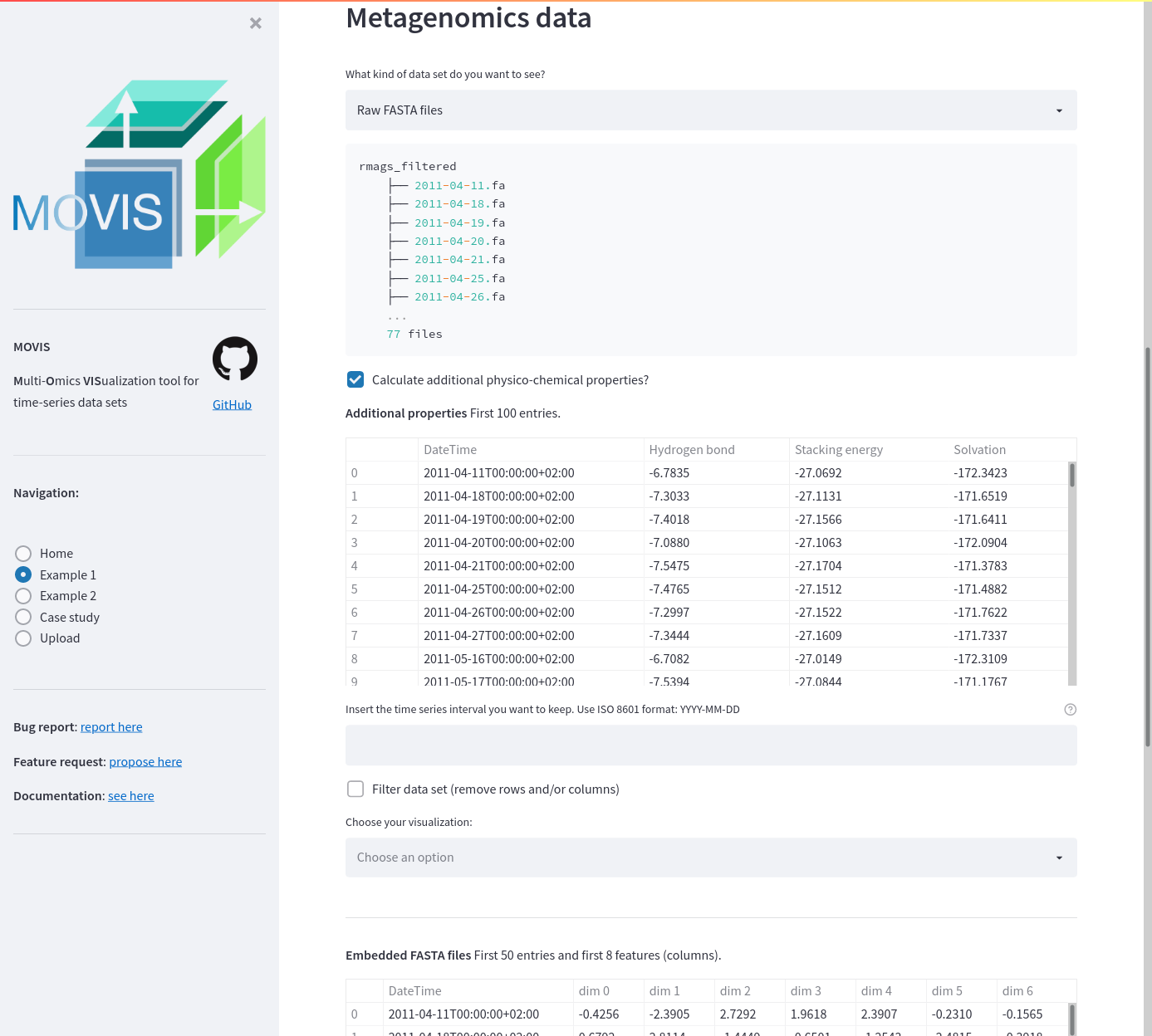
Example data 1. The screenshot shows additional physico-chemical properties calculated and displayed to the user. The first 50 entries of the embedded FASTA files are also displayed.

Genomics filtering on Example data 1. A filtering step is added to slice the data from 2011-04-11 to 2011-04-27. Additionally, certain row numbers are omitted.
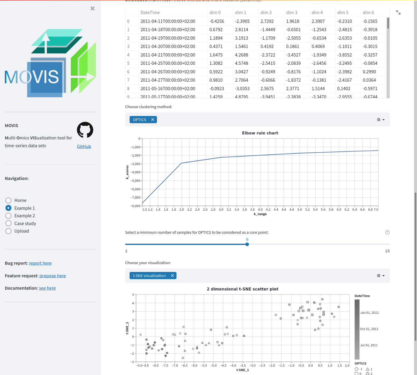
Embedding for Example data 1. The embedding of the resulting genomics data is displayed (50 first entries). A clustering method is applied: OPTICS. A threshold or minimum number of samples for the method is set using a slider. To evaluate the results in the high dimensional space, the t-SNE visualization is chosen.
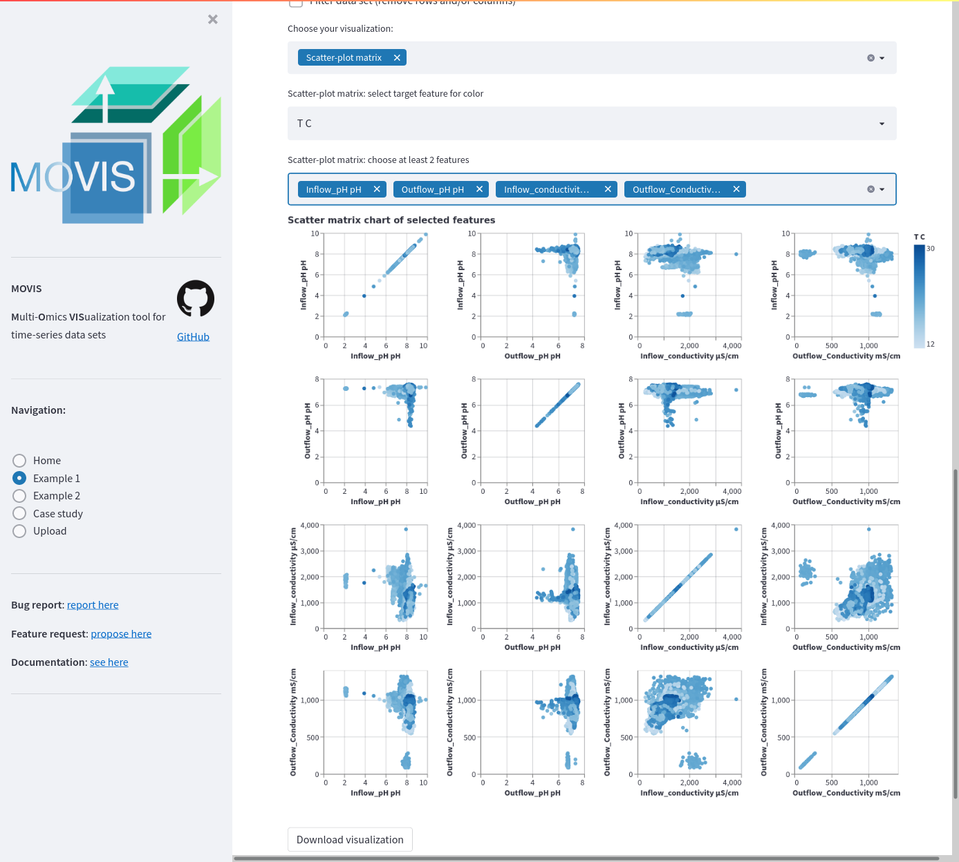
Scatter plot matrix for selected features in the physico-chemical data. Four features are selected: InflowpH, OutflowpH, Inflowconductivity, and Out-flowconductivity; totalling 16 possible scatter plot combinations which are displayed as a matrix using the small multiple idiom. A tooltip and a selection are available to investigate certain data points and their characteristics.
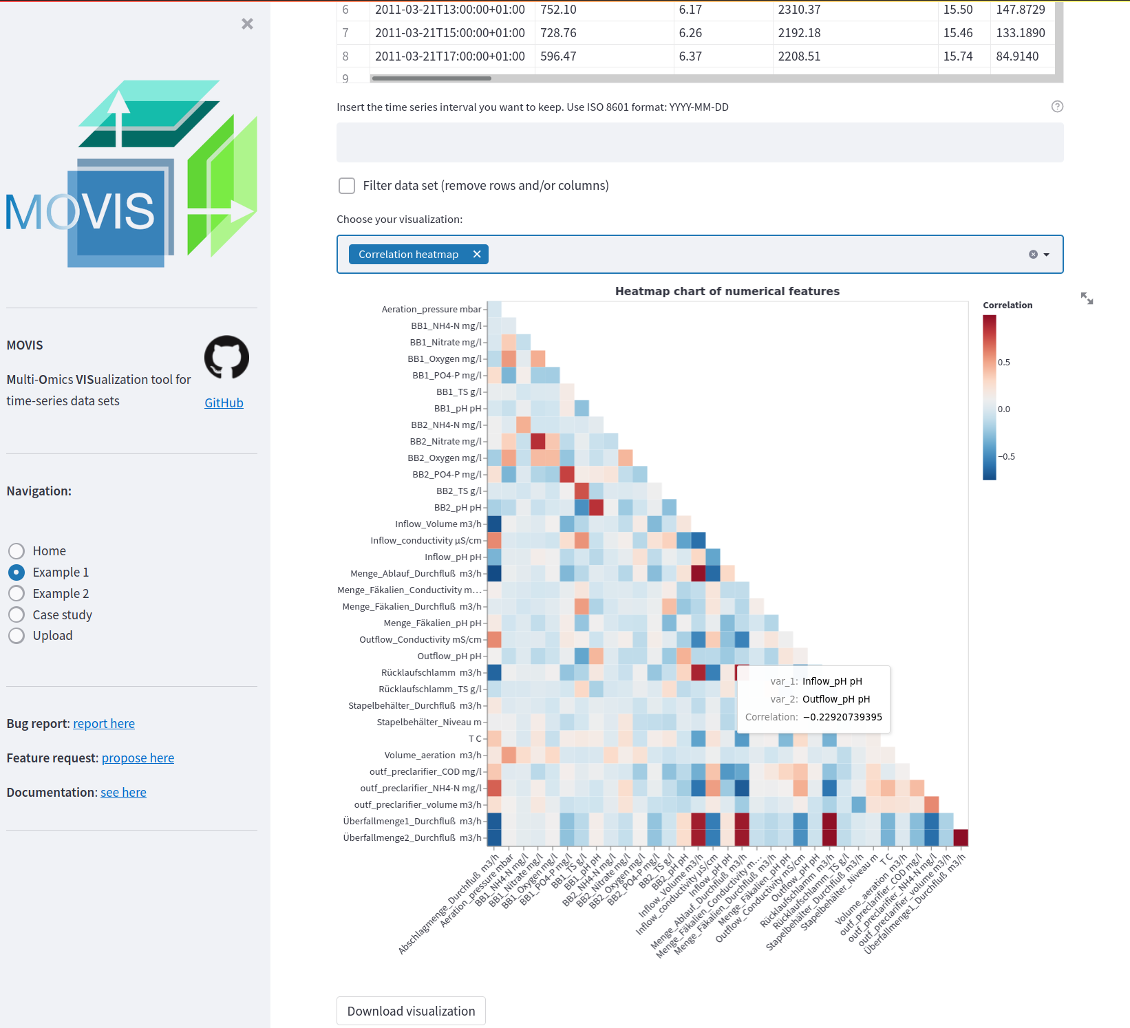
Triangular heatmap of all features in the physico-chemical properties data. A diverging color scheme palette is selected to showcase low and high correlations with less emphasis the mid-range values. A tooltip is available to investigate certain heatmap cells.
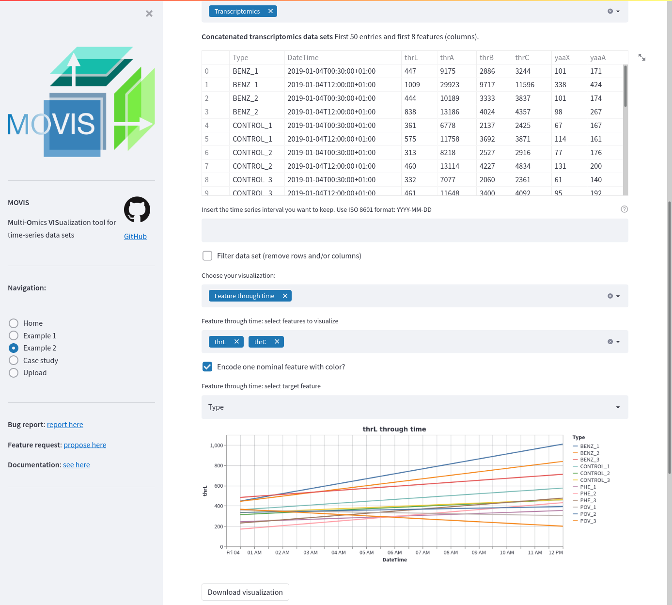
Example 2 transcriptomics data. A time-series of selected features is displayed as a line plot. Two features are selected: thrL and thrC. A categorical or nominal encoding is carried out for each of the 11 reported types. The Tableau 20 color palette is used.