Li Yang
-
$^1$ Department of Mechanical and Energy Engineering, Southern University of Science and Technology. -
$^2$ Department of Computer Science and Engineering, Southern University of Science and Technology.
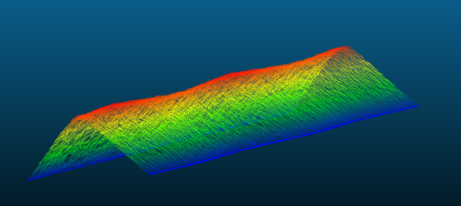
This project is based on the 3D point cloud of a grinding wheel modeled as shown in the figure below, aiming to estimate its radius.
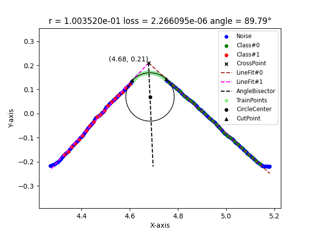
The algorithm aggregates the data near the y-axis through mean pooling, transforming it into a 2D plane problem and obtaining several batches. For each batch, it uses downsampling, DBSCAN clustering, and least squares fitting to obtain the boundary equations of the two straight lines on both sides. Then, using the original data on the angle bisector, it estimates the circle through gradient descent using the MSE loss function. Finally, for each batch of data, it reports the estimated radius of the circle.
First, use conda to install a virtual environment named corfit and configure all the required packages for the code.
(base) $ git clone https://github.com/Maystern/WheelRadiusPointCloud.git
(base) $ cd WheelRadiusPointCloud
(base) $ conda create -n corfit python=3.7.16
(base) $ conda activate corfit
(corfit) $ pip install -r requirements.txt
Check if the project is configured in the following format:
.
├── data
├── pic
├── results
├── README.md
├── main.py
└── requirements.txt
Place the raw data files in CSV format that need to be processed in the ./data directory, such as sample.csv.
- Note: You can directly download our test data sample (
sample.csv) from Tencent Weiyun using the following link: https://share.weiyun.com/1Azqvb3Y. Furthermore, to fortify the robustness of this project, additional test cases will be integrated in subsequent updates.
The format of the sample.csv file should be as follows, including headers, the number of points, and data separated by spaces:
//X Y Z
270385
4.28700018 0.00000000 -0.21818000
4.28999996 0.00000000 -0.21731000
4.29300022 0.00000000 -0.21613000
4.29600000 0.00000000 -0.21573000
4.29899979 0.00000000 -0.21510001
4.30200005 0.00000000 -0.21681000
4.38600016 0.00000000 -0.11171000
4.38899994 0.00000000 -0.10954000
4.39200020 0.00000000 -0.10778000
4.39499998 0.00000000 -0.10637000
4.39799976 0.00000000 -0.10401000
...
You can use visualization tools like CloudCompare to load and inspect the processed point cloud data.
To run the code, use the following command: python main.py -n sample.csv (where the -n parameter is mandatory, and other parameters have default values that can be modified). For detailed information on other parameters, you can refer to python main.py --help.
(corfit) $ python main.py -h
usage: main.py [-h] [-n CORNER_EXAMPLE_NAME] [-pic PIC_STORE_NAME]
               [-result RESULT_STORE_NAME] [-i EXPECTED_INTERVAL_COUNT]
               [-d DOWNSAMPLING_FACTOR] [-w LINE_FITTING_WINDOW_SIZE]
               [-s RANDOM_SEED] [-dbcan_eps DBSCAN_EPS]
               [-dbcan_min_sample DBSCAN_MIN_SAMPLE] [-l LEARNING_RATE]
               [-e EPSILON] [-r PRIOR_CIRCLE_R]

Estimation of Grinding Wheel Radius Using Gradient Descent Algorithm Based on
CSV Point Cloud Data.

optional arguments:
  -h, --help            show this help message and exit
  -n CORNER_EXAMPLE_NAME
                        [default: None | str] source data CSV file name, which
                        should be placed in the ./data folder.
  -pic PIC_STORE_NAME   [default: pic | str] output image folder name, which
                        should be placed in the project root directory ./
  -result RESULT_STORE_NAME
                        [default: results | str] output results folder name,
                        which should be placed in the root directory ./
  -i EXPECTED_INTERVAL_COUNT
                        [default: 10 | int] aggregation factor for y, how many
                        neighboring y values to calculate R at a time.
  -d DOWNSAMPLING_FACTOR
                        [default: 5 | int] downsampling factor, determining a
                        point for estimating the lines on both sides every few
                        data points.
  -w LINE_FITTING_WINDOW_SIZE
                        [default: 5 | int] number of points in the sliding
                        window, consecutively fitting lines with multiple
                        downsampling points to calculate the normal vector.
  -s RANDOM_SEED        [default: 42 | int] random seed
  -dbcan_eps DBSCAN_EPS
                        [default: 0.05 | float] radius size of the
                        neighborhood for DBSCAN.
  -dbcan_min_sample DBSCAN_MIN_SAMPLE
                        [default: 5 | int] minimum number of members in a
                        cluster for DBSCAN.
  -l LEARNING_RATE      [default: 0.01 | float] learning rate for gradient
                        descent using Adam.
  -e EPSILON            [default: 1e-08 | float] Termination criterion for
                        gradient descent, |loss' - loss| < epsilon
  -r PRIOR_CIRCLE_R     [default: 1.0 | float] Prior circle radius, which is
                        used to set the initial value for gradient descent in
                        estimating the original radius of the grinding wheel.
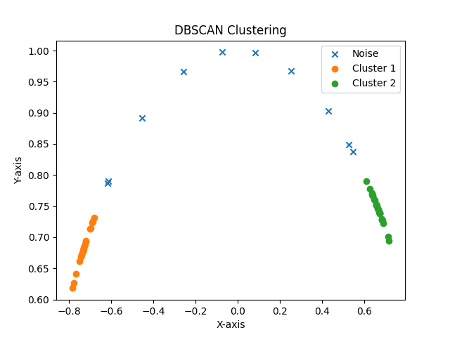
You can view the results of DBSCAN clustering and the fitting calculation for this batch in the ./pic/sample/batch_id directory, as shown in the following images:
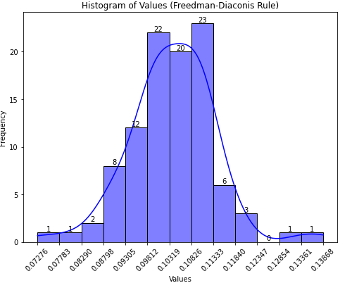
Once the progress bar completes, you will find all batch fitting results (radius, angle between fitted lines) and a visualized histogram in the ./results/sample folder, as illustrated below:
// results.csv
Block,R,Angle
1,0.11148012358179621,89.90166948614373
2,0.1003519830657477,89.79184732861077
3,0.10538032984418592,89.55709871217091
4,0.1024437819096742,89.9580235832247
5,0.11876593782266195,89.8372186694736
6,0.10789719614089213,89.79062547012468
7,0.10562980246049125,89.67696872640295
8,0.11557501790091716,89.55541525935509
9,0.11232309985505863,89.9113023350095
10,0.11259368715129213,90.22478354468474
11,0.09691442408830694,89.62875472888935
...