-
Notifications
You must be signed in to change notification settings - Fork 137
BSD Calibration Values
NOTE: The below information is outdated. The calibration model is a little different than presented here. See survive_reproject.c for code.
Much like with cameras, lighthouses in practice are non-ideal systems. Unlike standard cameras, there is no canonical 'fish eye' or 'pin hole' camera models you can reference. The purpose of this page is two fold: to describe the general way in which you can calibrate a lighthouse, and to also describe the explicit way you can use the BSD calibration data to get more precise angles from the lighthouse.
Nairol basically describing the entire thing
As with calibration models, the error is best described as deviations from the ideal rather than in how to correct those deviations. Again, as with cameras, this is typically good enough to apply optimization models that minimize reprojection error. Our parameterization for the calibration of a lighthouse as described by nairol is:
| Name | Description | Deviation |
|---|---|---|
| phase[2] | Constant offset from ideal on x and y | Δx = phase[0] |
| tilt[2] | Measure of 'tilt', expressed in radians. | Δx ~ tan(tilt[0]) * y |
| curve[2] | Measure of non-linear deviation across the sweep plane | Δx ~ curve[0] * y * y. |
| gibpha[2] gibmag[2] |
First fourier term for the correction. See here | Δx = sin(x + gibpha[0]) * gibmag[0] |
For our reprojection model, we start with knowing X, Y, and Z of the point in space. Assume the lighthouse is at origin. We can easily calculate the point on a plane which the ray from the lighthouse passes through to intersect [X, Y, Z]:
x = -x / -z
y = y / -z
Note the signs are basically arbitrary and represented here to be consistent with libsurvives specification of the state space of a lighthouse.
From this we can calculate the idealized angle we would see in a perfect lighthouse:
ideal_angle[0] = atan(x)
ideal_angle[1] = atan(y)
Finally we have what we expect to see given the calibration values:
observed_angle[0] = ideal_angle[0] - phase[0] - tan(tilt[0]) * y - curve[0] * y * y - sin(gibPhase[0] + ideal_angle[0]) * gibMag[0]
observed_angle[1] = ideal_angle[1] - phase[1] - tan(tilt[1]) * x - curve[0] * x * x - sin(gibPhase[1] + ideal_angle[1]) * gibMag[1]
Some notes about this set of equations: There are a number of permutations to this system that could work for a calibration model. All the minuses could be pluses, the sin could be cos, tan(tilt[0]) could just be the calculated constant -- in which case its just the slope of the line in terms of ax + b = c and in general you could change the units / offset of all values arbitrarily and still have a system which could serve as a calibration scheme.
The choices here are not arbitrary however, they reflect what we've found to best match the calibration values from the lighthouse.
In general terms, depending on parameter values, solving for the exact ideal_angle algebraically isn't typically feasible:
x = tan(ideal_angle[0])
y = tan(ideal_angle[1])
ideal_angle[0] = observed_angle[0] + phase[0] + tan(tilt[0]) * y + curve[0] * y * y + sin(gibPhase[0] + ideal_angle[0]) * gibMag[0]
ideal_angle[1] = observed_angle[1] + phase[1] + tan(tilt[1]) * x + curve[0] * x * x + sin(gibPhase[1] + ideal_angle[1]) * gibMag[1]
Note that this defines ideal_angle in terms of ideal_angle which makes solving it exactly sort of gross.
But, in practical terms, most calibrations tend to follow a pattern where each successive term handles ~90% of the remaining error and that seems here true -- just accounting for phase gives very useful values right out of the gate. And if we look at the above formulation as a recursive sequence, we can hand-waveingly conclude that this sequence will converge to ideal_angle since at every iteration of the sequence each term changes a little less each time.
We also know a very good approximation to start with since the phase removes such a large portion of the reprojection error. The exact formulation of this is:
ideal_angle(0)[0] = observed_angle[0] + phase[0]
ideal_angle(0)[1] = observed_angle[1] + phase[1]
x(t) = tan(ideal_angle(t)[0])
y(t) = tan(ideal_angle(t)[1])
ideal_angle(t)[0] = observed_angle[0] + phase[0] + tan(tilt[0]) * y(t-1) + curve[0] * y(t-1) * y(t-1 + sin(gibPhase[0] + ideal_angle(t-1)[0]) * gibMag[0]
ideal_angle(t)[1] = observed_angle[1] + phase[1] + tan(tilt[1]) * x(t-1) + curve[0] * x(t-1) * x(t-1) + sin(gibPhase[1] + ideal_angle(t-1)[1]) * gibMag[1]
In theory, the error term at t is dependent on the calibration values themselves. In practice, we've found that just solving for t = 4 is sufficiently accurate.
There are a number of ways to solve for this model. The most straight forward mathematically is to construct something you know the exact dimensions to, take a bunch of readings when you know where that object is in space, and then solving for those terms using some technique like bundle adjustment to iteratively lower the reprojection error.
Since vive tracked objects store their exact sensor locations relative to their origin, that saves you precision cutting something.
Knowing the exact location in space is a little more difficult; most of the reason we want to be able to use calibration data is to more precisely solve for that. Two things work in our favor for this:
- Two lighthouses at two different orientations are going to have vastly different error modes. In general, if you are able to aggregate the data from both lighthouses the error you accrue from not having a calibrated lighthouse will tend to cancel itself out the more lighthouse-sensor pairs you know. This is basically how SBA solver worked before any calibration data was used.
- Iteratively bootstraping calibrations from positions and positions from calibrations is basically what bundle adjustment does. Model the lighthouses as pose + calibration value (17 unknowns per) and the object in space is at origin. This gives 34 unknowns. If you take a snapshot of the light data of the object just standing still, you need just 9 sensors out of the ~20ish on an object to solve that iteratively. Obviously more is better, and in practice a good setup should give you ~30 xy pairs (15 sensors seen from each lighthouse, giving 60 measurements). You can also take multiple snapshots for more accurate results.
For our purposes though, this data is already stored in the lighthouse and having to calibrate every lighthouse you want to use would be annoying if you knew exactly what you were doing, and potentially incredibly frustrating if you didn't. So our aim is to not do any of this in libsurvive, and figure out a way to use the existing calibration values.
Obviously, for perfect calibration we'd want to know and use the vives exact formulation -- down to their choice of signs, offsets, scales, etc.
If our goal though is just to get arbitrarily close, we can approximate these formulations. The first thing we do is add a scalar term to each parameter.
We do this for two reasons -- first it gives us a way to flip the bit on any given value.
But secondly, we are operating under an assumption that an ideal camera model would have zeros across the board for its calibration parameter. This is a pretty good assumption practically speaking -- the only reason to not do this would be obfuscation, and if they particularly cared to obfuscate things config data wouldn't be available for the sensors in JSON.
If we start each parameter at a very low value -- say 1/100000 -- we can calculate the reprojection error over a variety of datasets and figure out if it added error or took some away. If it added error, we invert the value and run it again. So long as our formulations are positively correlated with the formulations that valve used, we can tweak these values towards greater magnitudes until, at some point, we overcorrect and increase the reprojection error in some cases.
Since the calibration parameters aren't orthogonal to eachother, each should be brought up slowly in turn. When we found inconsistencies, we changed our formulation to another one that would address the same error source but wasn't entirely positively correlated -- for instance, swapping cos with sin, or swapping tilt with tan(tilt).
After a lot of trial and error and moving an HMD across the floor very slowly, this is our current formulation and scale coefficients:
observed_angle[0] = ideal_angle[0] - scale_phase * phase[0] - tan(scale_tilt * tilt[0]) * y - scale_curve * curve[0] * y * y - scale_gib * sin(gibPhase[0] + ideal_angle[0]) * gibMag[0]
observed_angle[1] = ideal_angle[1] - scale_phase * phase[1] - tan(scale_tilt * tilt[1]) * x - scale_curve * curve[0] * x * x - scale_gib * sin(gibPhase[1] + ideal_angle[1]) * gibMag[1]
scale_phase = 1.0;
scale_tilt = 1. / 10.;
scale_curve = 1. / 10;
scale_gib = -1. / 10;
The fact that these aren't all of magnitude one means there is some assumption about units that is wrong, or more likely, that one or more of our formulations isn't identical. From all the datasets, it seems likely that they are all positively correlated; and even so we have managed to reduce our error from the substantial uncalibrated error to the difference in one of the above functions with the actual valve formulation. In practice, at some point this error is arbitrary and insignificant when it is on the same order as noise.
These parameters were tuned with data from 4 lighthouses. I suspect that it is possible that it overfit to that set of 4. If this calibration parameter set makes your system perform worse, please, please submit an issue and upload a playback file which starts with the HMD in the middle of your space, let it sit for 15 seconds and then slowly try to move it around the whole space -- the goal is for it to appear in the corners of the lighthouse at some point in the playback. It doesn't have to be terribly long. This would be a big help to tuning these systems.
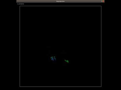
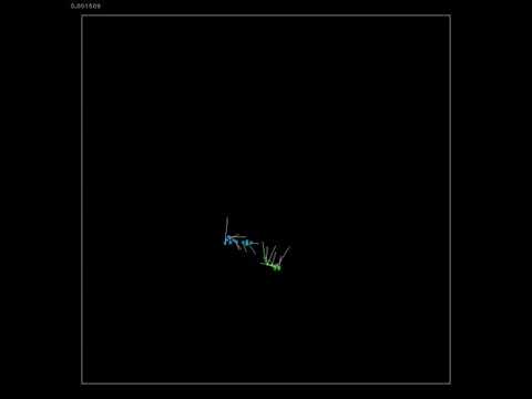
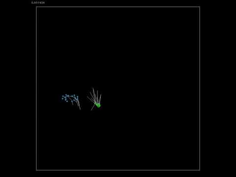
A good way to intuitively understand what reprojection error is, is to watch it. The number at the top is a running reprojection error in radians. The videos are sped up by about 50%.
In this video, we run EPNP over wholly uncalibrated angles. Circles are were the measurements are, and the squares are where the reprojection puts them at. This implementation can't integrate information from two lighthouses and so naturally is very susceptible to any calibration error. You can basically see the phase offset.
Notice SBA, able to integrate data from both lighthouses, does a very good job without calibration information available as it is able to basically average the resulting error out. White lines had to be added when the reprojection and measured point overlap on screen to still a representation of the error. This line is 10000x as long as the actual error.
You can start to see patterns, particularly around the edges. You can also see how much error is generated based on motion -- the X and Y sweep pattern are 16ms apart, and so the object basically is placed in the middle and there is error on both sides.
Phase calibration values being integrated helps massively; the error terms are more clustered and you can start to see patterns in reprojection error on the outside edge of the frame. Note that the reprojection error is roughly 5x higher with no phase calibration.
Using the LH calibration, most of the time when the object is stationary even the 10k magnified line disappears. Occasionally you can see a pattern that might indicate where there is error between our formulation and the hardware one. This gives roughly 15% better reprojection numbers.
A good way to think of calibration is that for every possible valid value, there is a mapping to another, nearby, value. We can actually draw this:

Obviously this image changes based on parameter values of the lighthouse.
The wheel at the top left indicates the direction of a particular color hue. The relative intensities indicate how far away the source point is. Absolute black means no displacement; and an ideal lighthouse would just be a black screen. Note that this image doesn't have phase in it -- if it did, all you would see is the phase since it's so much more impactful than anything else.
We can break this image down into it's equivalent parts.

Since phase is a constant offset, its just a single constant color.


