Quantum Mechanics is considered as one of the most weird branches in physics with the most, although accurate, counterintuitive predictions. The problem lies not on the theory but on what it is trying to explain: the microscopic world. Moreover, due to the complicated form of the Schrödinger equation, there are only few examples where it exists an analytical solution to the problem.
Therefore, the motivation of this repository is to explore the incredible effects of Quantum Mechanics solving the Schrödinger equation numerically under different potentials. The programs allows to obtain the eigenvalues, eigenstates and a temporal evolution of the probability density of a particle for the potential introduced by the user.
As for the numerical system precision, the method has been stressed to find out its precision and the method is used for two real models: the ammonia molecule and the hydrogen atom.
This repository offers the open-source python 2.7 programs to solve the Schrödinger equation under arbitrary potentials. It is designed to be implemented through Jupiter Notebook, to ease user's experience and facilitate working with arbitrary potentials.
https://gmegh.github.io/Quantum_PEF2/
Download the programs as a zip and install Jupyter Notebook. Then run the general_main.ipynb and introduce the arbitrary potential with which you want to work. Remind that the only block which has to be modified is the first one. Should you were to modify deeper code or other blocks, this may trigger malfunctions to the program. An mp4 file is produced with the temporal evolution.
For detailed instructions go to: README_Instructions.md
An good example is the double potential:
https://www.youtube.com/watch?v=m3_smsdw8Kk
The Richardson method used in calculating the eigenvalues, ensures a rapid, robust and accurate results. Furthermore, the program has been numerically stressed out with different high-dificulty potentials, such as the Poschl-Teller modified potential.
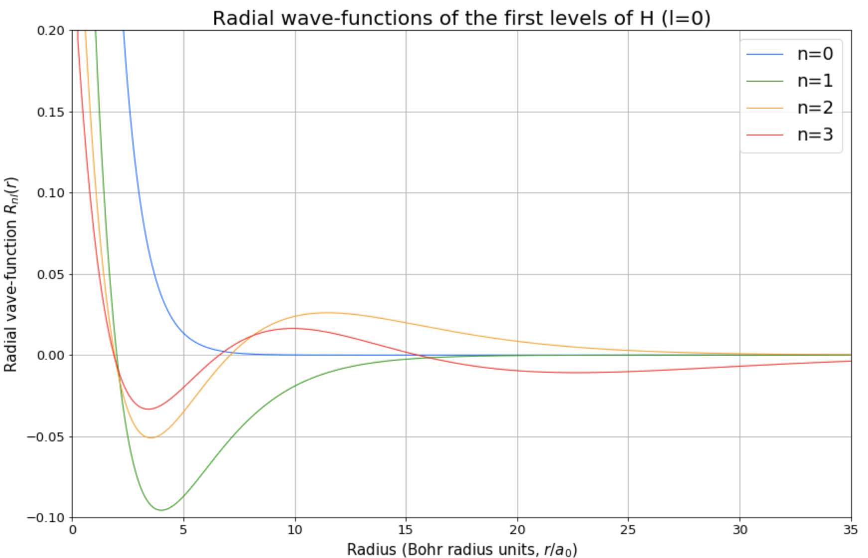
Furthermore, it is also presented a real-case application, which allows to study the radial wave-function of the Hydrogen atom through the three-dimensional case. Choosing the azimuthal quantum number l, the user will obtain a plot of both: the radial wave-function and the radial probability density function for the first four eigenstates.
For instance, for l = 0 one of the obtained figures is the following,
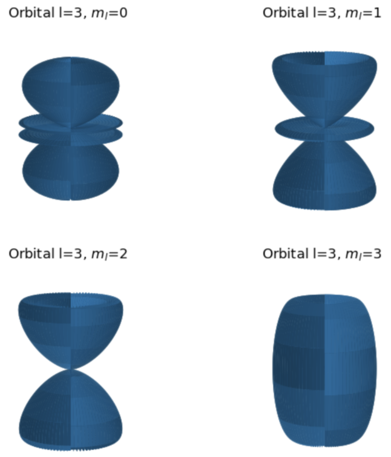
The angular wave-function is also obtained, in this case, through the analytic expression and is represented in a polar plot and 3D to show the shape of electron orbitals in H atom. This is done for an arbitrary value of the azimuthal quantum number l which is the input of the user to the program. For instance, for l=3, the orbitals plot which is obtained is:

