Weighted gradient matrix

The module WeightedGradient.py contains a function for computing a weighted gradient matrix. Using the weighted gradient matrix, the gradient of a P1 Function may be computed very fast using merely a single matrix vector product. The gradient can be computed on a continuous Lagrange space of any degree.

from dolfin import *
from fenicstools.WeightedGradient import weighted_gradient_matrix

mesh = UnitSquareMesh(10, 10)
V = FunctionSpace(mesh, "CG", 1)

# Set an exact solution
p = interpolate(Expression("sin(x[0])*cos(x[1])"), V)
dpdxe = interpolate(Expression("cos(x[0])*cos(x[1])"), V)
dpdye = interpolate(Expression("-sin(x[0])*sin(x[1])"), V)

# Compute gradient of p on V
dP = weighted_gradient_matrix(mesh, (0, 1), 1)
dpdx = Function(V)
dpdy = Function(V)
dpdx.vector()[:] = dP[0]*p.vector()
dpdy.vector()[:] = dP[1]*p.vector()

# Compute gradient using regular projection
dpdxp = project(p.dx(0), V)
dpdyp = project(p.dx(1), V)

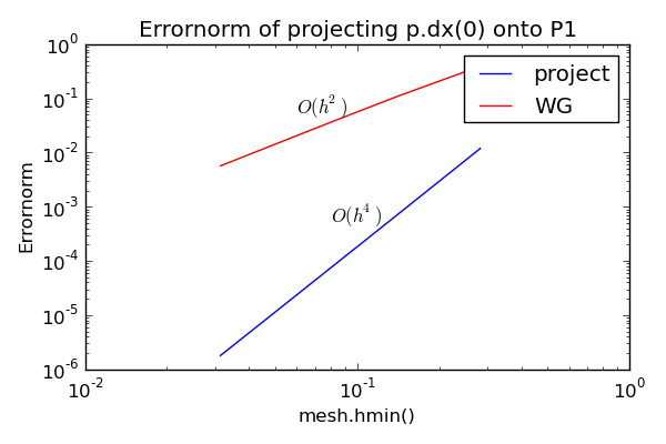
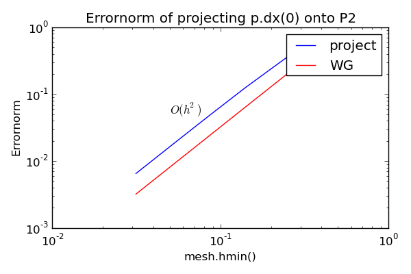
The accuracy of the weighted gradient matrix is investigated using the following script that is periodic to eliminate boundary effects.

from dolfin import *
from pylab import loglog, show, legend, title, xlabel, text, ylabel, figure
from fenicstools.WeightedGradient import weighted_gradient_matrix
        
class PeriodicDomain(SubDomain):

    def inside(self, x, on_boundary):
        return bool((near(x[0], 0) or near(x[1], 0)) and 
            (not ((near(x[0], 0) and near(x[1], 2)) or 
                    (near(x[0], 2) and near(x[1], 0)))) and on_boundary)

    def map(self, x, y):
        if near(x[0], 2) and near(x[1], 2):
            y[0] = x[0] - 2.0
            y[1] = x[1] - 2.0
        elif near(x[0], 2):
            y[0] = x[0] - 2.0
            y[1] = x[1]
        else:
            y[0] = x[0]
            y[1] = x[1] - 2.0

constrained_domain = PeriodicDomain()
for vel_deg in (1, 2): # Loop over two degrees in FunctionSpace interpolated to
    err_reg = []
    err_wg = []
    hmin = []
    for N in range(10, 100, 10): # Loop over different mesh sizes
        mesh = RectangleMesh(0, 0, 2, 2, N, N)
        Q = FunctionSpace(mesh, "CG", 1, constrained_domain=constrained_domain) 
        V = FunctionSpace(mesh, "CG", vel_deg, constrained_domain=constrained_domain)  
        u = TrialFunction(V)
        v = TestFunction(V)

        # Exact solution
        p = interpolate(Expression("sin(pi*x[0])*cos(pi*x[1])"), Q)
        dp_exact = interpolate(Expression("pi*cos(pi*x[0])*cos(pi*x[1])"), V)
        dp_exact.update()

        # Compute regular projection
        dp_regular = project(p.dx(0), V)

        # Compute solution using weighted gradient matrix
        dP = weighted_gradient_matrix(mesh, 0, vel_deg, constrained_domain=constrained_domain)
        dp_wg = Function(V)
        dp_wg.vector()[:] = dP * p.vector() 

        # Compute error
        err_reg.append(errornorm(dp_regular, dp_exact, degree_rise=0))
        err_wg.append(errornorm(dp_wg, dp_exact, degree_rise=0))
        hmin.append(mesh.hmin())

    # Plot the errornorms
    figure()
    loglog(hmin, err_reg, 'b')
    loglog(hmin, err_wg, 'r')

    legend(("project", "WG"))
    title("Errornorm of projecting p.dx(0) onto P{}".format(vel_deg))
    ylabel("Errornorm")
    xlabel("mesh.hmin()")
    if vel_deg == 1:
        text(0.08, 5e-4, "$O(h^4)$")
        text(0.06, 0.05, "$O(h^2)$")
    else:
        text(0.06, 0.05, "$O(h^2)$")
        
show()

The error plots are shown below. Due to superconvergence the regular project function reaches a whopping 4th order accuracy for this problem on P1 elements because of the regular size and alignment of the mesh. A skewed mesh or "crossed" type reduces the order to 2 also for the regular project function.