Swapping in SEPP for read placement with q2 picrust2
If you do not have at least 20GB of RAM, the best alternative is to use a different read placement program for the read placement step. This tutorial will demonstrate how ASVs placed with q2-fragment-insertion can be used as input to the q2-picrust2 plugin.
You can see a description of the PICRUSt2 command by running:
qiime picrust2 custom-tree-pipeline --help
The required inputs are --i-table and --i-tree, which need to correspond to QIIME2 artifacts of types FeatureTable[Frequency] and Phylogeny[Rooted], respectively. The Feature Table needs to contain the abundances of ASVs (i.e. a BIOM table) and the tree file needs to contain the ASVs placed into the PICRUSt2 reference tree.
We will be using test files from the PICRUSt2 tutorial for this example. You can download these files using the below commands:
mkdir q2-picrust2_test

cd q2-picrust2_test

wget http://kronos.pharmacology.dal.ca/public_files/tutorial_datasets/picrust2_tutorial_files/mammal_biom.qza

wget http://kronos.pharmacology.dal.ca/public_files/tutorial_datasets/picrust2_tutorial_files/mammal_seqs.qza

wget http://kronos.pharmacology.dal.ca/public_files/tutorial_datasets/picrust2_tutorial_files/mammal_metadata.tsv
These files correspond to the ASV count table, ASV sequences, and metadata for the samples. There are 11 samples and 371 ASVs in total. These samples were collected from the mammalian stool of Arctic wolves, coyotes, beavers, and porcupines, as previously described.
To place the ASVs we will first run q2-fragment-insertion against the PICRUSt2 reference multiple-sequence alignment and phylogeny. Note that using this sequence placement approach differs from the default PICRUSt2 pipeline, but is easier to integrate with the QIIME2 framework. Note that you need to place your ASVs into the PICRUSt2 reference files - if you place your ASVs into the default SEPP reference files you will get downstream errors. The two reference files used here are the same ones you would use with your own data. Download the reference files and place the study sequences into the tree:
wget http://kronos.pharmacology.dal.ca/public_files/tutorial_datasets/picrust2_tutorial_files/reference.fna.qza

wget http://kronos.pharmacology.dal.ca/public_files/tutorial_datasets/picrust2_tutorial_files/reference.tre.qza

qiime fragment-insertion sepp --i-representative-sequences mammal_seqs.qza \
                              --p-threads 1 --i-reference-alignment reference.fna.qza \
                              --i-reference-phylogeny reference.tre.qza \
                              --output-dir tutorial_placed_out
Now that we have our placed ASVs we can run qiime picrust2 custom-tree-pipeline. There are many options available for the standalone PICRUSt2 version, but currently only selecting the number of threads (--p-threads), hidden-state prediction (HSP) method (--p-hsp-method), and maximum NSTI value (--p-max-nsti) are specified.
The --p-max-nsti option specifies how distantly placed a sequence needs to be in the reference phylogeny before it is excluded. The default cut-off is 2. In human datasets used for testing PICRUSt2 the only ASVs above this default cut-off were 18S sequences erroneously in 16S datasets, which suggests this cut-off is highly lenient. For environmental datasets a higher proportion of ASVs may be thrown out based on this default cut-off (Douglas et al. In Prep).
You can run the full PICRUSt2 pipeline with this command (should take ~17 min and 5GB of RAM - this will be much faster if you can set more threads). Note in this case the pic the phylogenetic independent contrast hidden-state prediction method is indicated since it is fastest. However, we recommend that in practice users use the mp method (~40 min on 1 thread for this example).
qiime picrust2 custom-tree-pipeline --i-table mammal_biom.qza \
                                    --i-tree tutorial_placed_out/tree.qza \
                                    --output-dir q2-picrust2_output \
                                    --p-threads 1 --p-hsp-method pic \
                                    --p-max-nsti 2
The output artifacts of this command are the red boxes in the flowchart here. In addition, MetaCyc pathway coverages will also be output, which could help advanced users interpret the pathway completeness, but will not be used by most users.
These output files in (q2-picrust2_output) are:
-
ec_metagenome.qza- EC metagenome predictions (rows are EC numbers and columns are samples). -
ko_metagenome.qza- KO metagenome predictions (rows are KOs and columns are samples). -
pathway_abundance.qza- MetaCyc pathway abundance predictions (rows are pathways and columns are samples). -
pathway_coverage.qza- MetaCyc pathway predicted coverages (rows are pathways and columns are samples).
The artifacts are all of type FeatureTable[Frequency], which means they can be used with QIIME2 plugins that process and analyze these datatypes.
For instance, you can get a summary of the pathway abundance file with this command, which you can view like any QIIME2 visualization.
qiime feature-table summarize --i-table q2-picrust2_output/pathway_abundance.qza --o-visualization q2-picrust2_output/pathway_abundance.qzv
You should see a table like this which describes the total pathway abundance per-sample (as well as other useful summaries):

The above metagenome predictions can be integrated into a number of QIIME2 analysis. For instance, you can quickly calculate diversity metrics based on these tables. The minimum sample pathway abundance found above was 239231, so we will rarify to this cut-off when calculating the core diversity metrics:
qiime diversity core-metrics --i-table q2-picrust2_output/pathway_abundance.qza --p-sampling-depth 239231 --m-metadata-file mammal_metadata.tsv --output-dir pathabun_core_metrics_out --p-n-jobs 1
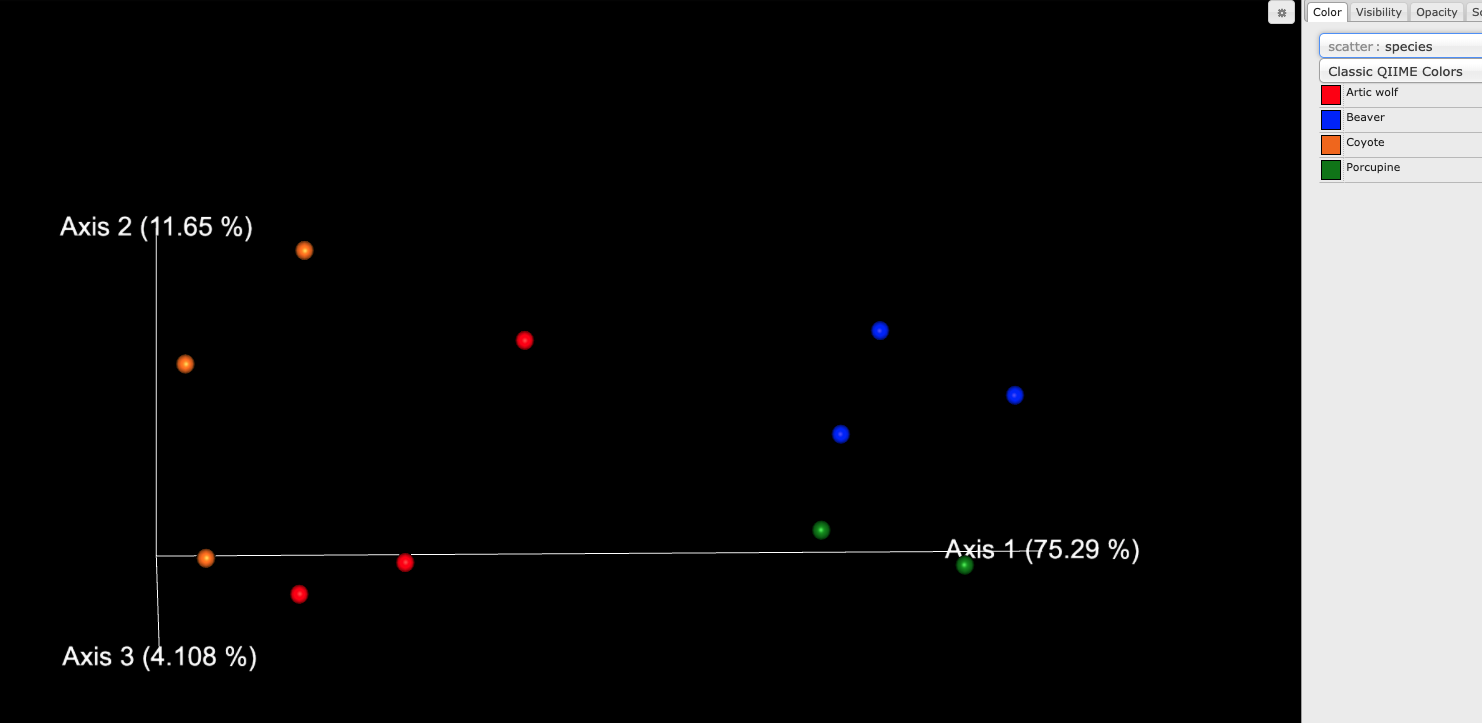
Take a look at pathabun_core_metrics_out/bray_curtis_emperor.qzv in the QIIME2 viewer. You should see a ordination plot like this, which shows how the clear difference between this dataset is between carnivores and rodents: