Release Release 0.18.0 · PennyLaneAI/pennylane

New features since last release

PennyLane now comes packaged with `lightning.qubit`

The C++-based lightning.qubit device is now included with installations of PennyLane. (#1663)

The lightning.qubit device is a fast state-vector simulator equipped with the efficient adjoint method for differentiating quantum circuits, check out the plugin release notes for more details! The device can be accessed in the following way:

import pennylane as qml

wires = 3
layers = 2
dev = qml.device("lightning.qubit", wires=wires)

@qml.qnode(dev, diff_method="adjoint")
def circuit(weights):
    qml.templates.StronglyEntanglingLayers(weights, wires=range(wires))
    return qml.expval(qml.PauliZ(0))

weights = qml.init.strong_ent_layers_normal(layers, wires, seed=1967)

Evaluating circuits and their gradients on the device can be achieved using the standard approach:

>>> print(f"Circuit evaluated: {circuit(weights)}")
Circuit evaluated: 0.9801286266677633
>>> print(f"Circuit gradient:\n{qml.grad(circuit)(weights)}")
Circuit gradient:
[[[-9.35301749e-17 -1.63051504e-01 -4.14810501e-04]
  [-7.88816484e-17 -1.50136528e-04 -1.77922957e-04]
  [-5.20670796e-17 -3.92874550e-02  8.14523075e-05]]

 [[-1.14472273e-04  3.85963953e-02 -9.39190132e-18]
  [-5.76791765e-05 -9.78478343e-02  0.00000000e+00]
  [ 0.00000000e+00  0.00000000e+00  0.00000000e+00]]]

The adjoint method operates after a forward pass by iteratively applying inverse gates to scan backwards through the circuit. The method is already available in PennyLane's default.qubit device, but the version provided by lightning.qubit integrates with the C++ backend and is more performant, as shown in the plot below: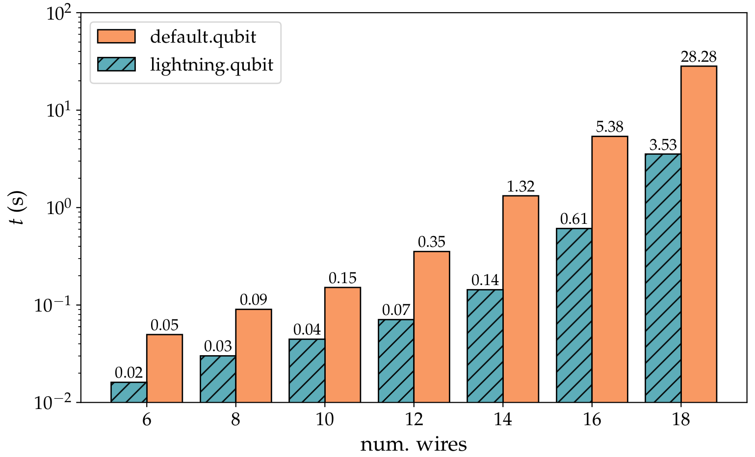

Support for native backpropagation using PyTorch

The built-in PennyLane simulator default.qubit now supports backpropogation with PyTorch. (#1360) (#1598)

As a result, default.qubit can now use end-to-end classical backpropagation as a means to compute gradients. End-to-end backpropagation can be faster than the parameter-shift rule for computing quantum gradients when the number of parameters to be optimized is large. This is now the default differentiation method when using default.qubit with PyTorch.

Using this method, the created QNode is a 'white-box' that is tightly integrated with your PyTorch computation, including TorchScript and GPU support.

x = torch.tensor(0.43316321, dtype=torch.float64, requires_grad=True)
y = torch.tensor(0.2162158, dtype=torch.float64, requires_grad=True)
z = torch.tensor(0.75110998, dtype=torch.float64, requires_grad=True)

p = torch.tensor([x, y, z], requires_grad=True)
dev = qml.device("default.qubit", wires=1)

@qml.qnode(dev, interface="torch", diff_method="backprop")
def circuit(x):
    qml.Rot(x[0], x[1], x[2], wires=0)
    return qml.expval(qml.PauliZ(0))

res = circuit(p)
res.backward()

>>> res = circuit(p)
>>> res.backward()
>>> print(p.grad)
tensor([-9.1798e-17, -2.1454e-01, -1.0511e-16], dtype=torch.float64)

Improved quantum optimization methods

The RotosolveOptimizer now can tackle general parametrized circuits, and is no longer restricted to single-qubit Pauli rotations. (#1489)

This includes:

layers of gates controlled by the same parameter,
controlled variants of parametrized gates, and
Hamiltonian time evolution.

Note that the eigenvalue spectrum of the gate generator needs to be known to use RotosolveOptimizer for a general gate, and it is required to produce equidistant frequencies. For details see Vidal and Theis, 2018 and Wierichs, Izaac, Wang, Lin 2021.

Consider a circuit with a mixture of Pauli rotation gates, controlled Pauli rotations, and single-parameter layers of Pauli rotations:

dev = qml.device('default.qubit', wires=3, shots=None)

@qml.qnode(dev)
def cost_function(rot_param, layer_par, crot_param):
    for i, par in enumerate(rot_param):
        qml.RX(par, wires=i)
    for w in dev.wires:
        qml.RX(layer_par, wires=w)
    for i, par in enumerate(crot_param):
        qml.CRY(par, wires=[i, (i+1) % 3])

    return qml.expval(qml.PauliZ(0) @ qml.PauliZ(1) @ qml.PauliZ(2))

This cost function has one frequency for each of the first RX rotation angles, three frequencies for the layer of RX gates that depend on layer_par, and two frequencies for each of the CRY gate parameters. Rotosolve can then be used to minimize the cost_function:

# Initial parameters
init_param = [
    np.array([0.3, 0.2, 0.67], requires_grad=True),
    np.array(1.1, requires_grad=True),
    np.array([-0.2, 0.1, -2.5], requires_grad=True),
]
# Numbers of frequencies per parameter
num_freqs = [[1, 1, 1], 3, [2, 2, 2]]

opt = qml.RotosolveOptimizer()
param = init_param.copy()

In addition, the optimization technique for the Rotosolve substeps can be chosen via the optimizer and optimizer_kwargs keyword arguments and the minimized cost of the intermediate univariate reconstructions can be read out via full_output, including the cost after the full Rotosolve step:

for step in range(3):
    param, cost, sub_cost = opt.step_and_cost(
        cost_function,
        *param,
        num_freqs=num_freqs,
        full_output=True,
        optimizer="brute",
    )
    print(f"Cost before step: {cost}")
    print(f"Minimization substeps: {np.round(sub_cost, 6)}")

Cost before step: 0.042008210392535605
Minimization substeps: [-0.230905 -0.863336 -0.980072 -0.980072 -1.       -1.       -1.      ]
Cost before step: -0.999999999068121
Minimization substeps: [-1. -1. -1. -1. -1. -1. -1.]
Cost before step: -1.0
Minimization substeps: [-1. -1. -1. -1. -1. -1. -1.]

For usage details please consider the docstring of the optimizer.

Faster, trainable, Hamiltonian simulations

Hamiltonians are now trainable with respect to their coefficients. (#1483)

from pennylane import numpy as np

dev = qml.device("default.qubit", wires=2)
@qml.qnode(dev)
def circuit(coeffs, param):
    qml.RX(param, wires=0)
    qml.RY(param, wires=0)
    return qml.expval(
        qml.Hamiltonian(coeffs, [qml.PauliX(0), qml.PauliZ(0)], simplify=True)
    )

coeffs = np.array([-0.05, 0.17])
param = np.array(1.7)
grad_fn = qml.grad(circuit)

>>> grad_fn(coeffs, param)
(array([-0.12777055,  0.0166009 ]), array(0.0917819))

Furthermore, a gradient recipe for Hamiltonian coefficients has been added. This makes it possible to compute parameter-shift gradients of these coefficients on devices that natively support Hamiltonians. (#1551)

Hamiltonians are now natively supported on the default.qubit device if shots=None. This makes VQE workflows a lot faster in some cases. (#1551) (#1596)
The Hamiltonian can now store grouping information, which can be accessed by a device to speed up computations of the expectation value of a Hamiltonian. (#1515)
```
obs = [qml.PauliX(0), qml.PauliX(1), qml.PauliZ(0)]
coeffs = np.array([1., 2., 3.])
H = qml.Hamiltonian(coeffs, obs, grouping_type='qwc')
```
Initialization with a grouping_type other than None stores the indices
required to make groups of commuting observables and their coefficients.
```
>>> H.grouping_indices
[[0, 1], [2]]
```

Create multi-circuit quantum transforms and custom gradient rules

Custom gradient transforms can now be created using the new @qml.gradients.gradient_transform decorator on a batch-tape transform. (#1589)

Quantum gradient transforms are a specific case of qml.batch_transform.

Supported gradient transforms must be of the following form:
```
@qml.gradients.gradient_transform
def my_custom_gradient(tape, argnum=None, **kwargs):
    ...
    return gradient_tapes, processing_fn
```
Various built-in quantum gradient transforms are provided within the qml.gradients module, including qml.gradients.param_shift. Once defined, quantum gradient transforms can be applied directly to QNodes:
```
>>> @qml.qnode(dev)
... def circuit(x):
...     qml.RX(x, wires=0)
...     qml.CNOT(wires=[0, 1])
...     return qml.expval(qml.PauliZ(0))
>>> circuit(0.3)
tensor(0.95533649, requires_grad=True)
>>> qml.gradients.param_shift(circuit)(0.5)
array([[-0.47942554]])
```
Quantum gradient transforms are fully differentiable, allowing higher order derivatives to be accessed:
```
>>> qml.grad(qml.gradients.param_shift(circuit))(0.5)
tensor(-0.87758256, requires_grad=True)
```
Refer to the page of quantum gradient transforms for more details.

The ability to define batch transforms has been added via the new @qml.batch_transform decorator. (#1493)

A batch transform is a transform that takes a single tape or QNode as input, and executes multiple tapes or QNodes independently. The results may then be post-processed before being returned.

For example, consider the following batch transform:

@qml.batch_transform
def my_transform(tape, a, b):
    """Generates two tapes, one with all RX replaced with RY,
    and the other with all RX replaced with RZ."""
    tape1 = qml.tape.JacobianTape()
    tape2 = qml.tape.JacobianTape()

    # loop through all operations on the input tape
    for op in tape.operations + tape.measurements:
        if op.name == "RX":
            with tape1:
                qml.RY(a * qml.math.abs(op.parameters[0]), wires=op.wires)
            with tape2:
                qml.RZ(b * qml.math.abs(op.parameters[0]), wires=op.wires)
        else:
            for t in [tape1, tape2]:
                with t:
                    qml.apply(op)

    def processing_fn(results):
        return qml.math.sum(qml.math.stack(results))

    return [tape1, tape2], processing_fn

We can transform a QNode directly using decorator syntax:

>>> @my_transform(0.65, 2.5)
... @qml.qnode(dev)
... def circuit(x):
...     qml.Hadamard(wires=0)
...     qml.RX(x, wires=0)
...     return qml.expval(qml.PauliX(0))
>>> print(circuit(-0.5))
1.2629730888100839

Batch tape transforms are fully differentiable:

>>> gradient = qml.grad(circuit)(-0.5)
>>> print(gradient)
2.5800122591960153

Batch transforms can also be applied to existing QNodes,

>>> new_qnode = my_transform(existing_qnode, *transform_weights)
>>> new_qnode(weights)

or to tapes (in which case, the processed tapes and classical post-processing functions are returned):

>>> tapes, fn = my_transform(tape, 0.65, 2.5)
>>> from pennylane.interfaces.batch import execute
>>> dev = qml.device("default.qubit", wires=1)
>>> res = execute(tapes, dev, interface="autograd", gradient_fn=qml.gradients.param_shift)
1.2629730888100839

Vector-Jacobian product transforms have been added to the qml.gradients package. (#1494)

The new transforms include:
- qml.gradients.vjp
- qml.gradients.batch_vjp

Support for differentiable execution of batches of circuits has been added, via the beta pennylane.interfaces.batch module. (#1501) (#1508) (#1542) (#1549) (#1608) (#1618) (#1637)

For now, this is a low-level feature, and will be integrated into the QNode in a future release. For example:

from pennylane.interfaces.batch import execute

def cost_fn(x):
    with qml.tape.JacobianTape() as tape1:
        qml.RX(x[0], wires=[0])
        qml.RY(x[1], wires=[1])
        qml.CNOT(wires=[0, 1])
        qml.var(qml.PauliZ(0) @ qml.PauliX(1))

    with qml.tape.JacobianTape() as tape2:
        qml.RX(x[0], wires=0)
        qml.RY(x[0], wires=1)
        qml.CNOT(wires=[0, 1])
        qml.probs(wires=1)

    result = execute(
        [tape1, tape2], dev,
        gradient_fn=qml.gradients.param_shift,
        interface="autograd"
    )
    return result[0] + result[1][0, 0]

res = qml.grad(cost_fn)(params)

Improvements

A new operation qml.SISWAP has been added, the square-root of the qml.ISWAP operation. (#1563)
The frobenius_inner_product function has been moved to the qml.math module, and is now differentiable using all autodiff frameworks. (#1388)
A warning is raised to inform the user that specifying a list of shots is only supported for QubitDevice based devices. (#1659)

The qml.circuit_drawer.MPLDrawer class provides manual circuit drawing functionality using Matplotlib. While not yet integrated with automatic circuit drawing, this class provides customization and control. (#1484)

from pennylane.circuit_drawer import MPLDrawer

drawer = MPLDrawer(n_wires=3, n_layers=3)

drawer.label([r"$|\Psi\rangle$", r"$|\theta\rangle$", "aux"])

drawer.box_gate(layer=0, wires=[0, 1, 2], text="Entangling Layers", text_options={'rotation': 'vertical'})
drawer.box_gate(layer=1, wires=[0, 1], text="U(θ)")

drawer.CNOT(layer=2, wires=[1, 2])
drawer.measure(layer=3, wires=2)

drawer.fig.suptitle('My Circuit', fontsize='xx-large')

The slowest tests, more than 1.5 seconds, now have the pytest mark slow, and can be selected or deselected during local execution of tests. (#1633)
The device test suite has been expanded to cover more qubit operations and observables. (#1510)
The MultiControlledX class now inherits from Operation instead of ControlledQubitUnitary which makes the MultiControlledX gate a non-parameterized gate. (#1557)
The utils.sparse_hamiltonian function can now deal with non-integer wire labels, and it throws an error for the edge case of observables that are created from multi-qubit operations. (#1550)
Added the matrix attribute to qml.templates.subroutines.GroverOperator (#1553)
The tape.to_openqasm() method now has a measure_all argument that specifies whether the serialized OpenQASM script includes computational basis measurements on all of the qubits or just those specified by the tape. (#1559)
An error is now raised when no arguments are passed to an observable, to inform that wires have not been supplied. (#1547)

The group_observables transform is now differentiable. (#1483)

For example:

import jax
from jax import numpy as jnp

coeffs = jnp.array([1., 2., 3.])
obs = [PauliX(wires=0), PauliX(wires=1), PauliZ(wires=1)]

def group(coeffs, select=None):
  _, grouped_coeffs = qml.grouping.group_observables(obs, coeffs)
  # in this example, grouped_coeffs is a list of two jax tensors
  # [DeviceArray([1., 2.], dtype=float32), DeviceArray([3.], dtype=float32)]
  return grouped_coeffs[select]

jac_fn = jax.jacobian(group)

>>> jac_fn(coeffs, select=0)
[[1. 0. 0.]
[0. 1. 0.]]

>>> jac_fn(coeffs, select=1)
[[0., 0., 1.]]

The tape does not verify any more that all Observables have owners in the annotated queue. (#1505)

This allows manipulation of Observables inside a tape context. An example is expval(Tensor(qml.PauliX(0), qml.Identity(1)).prune()) which makes the expval an owner of the pruned tensor and its constituent observables, but leaves the original tensor in the queue without an owner.
The qml.ResetError is now supported for default.mixed device. (#1541)
QNode.diff_method will now reflect which method was selected from diff_method="best". (#1568)
QNodes now support diff_method=None. This works the same as interface=None. Such QNodes accept floats, ints, lists and NumPy arrays and return NumPy output but can not be differentiated. (#1585)
QNodes now include validation to warn users if a supplied keyword argument is not one of the recognized arguments. (#1591)

Breaking changes

The QFT operation has been moved, and is now accessible via pennylane.templates.QFT. (#1548)
Specifying shots=None with qml.sample was previously deprecated. From this release onwards, setting shots=None when sampling will raise an error also for default.qubit.jax. (#1629)
An error is raised during QNode creation when a user requests backpropagation on a device with finite-shots. (#1588)
The class qml.Interferometer is deprecated and will be renamed qml.InterferometerUnitary after one release cycle. (#1546)
All optimizers except for Rotosolve and Rotoselect now have a public attribute stepsize. Temporary backward compatibility has been added to support the use of _stepsize for one release cycle. update_stepsize method is deprecated. (#1625)

Bug fixes

Fixed a bug with shot vectors and Device base class. (#1666)
Fixed a bug where @jax.jit would fail on a QNode that used qml.QubitStateVector. (#1649)
Fixed a bug related to an edge case of single-qubit zyz_decomposition when only off-diagonal elements are present. (#1643)
MottonenStatepreparation can now be run with a single wire label not in a list. (#1620)
Fixed the circuit representation of CY gates to align with CNOT and CZ gates when calling the circuit drawer. (#1504)
Dask and CVXPY dependent tests are skipped if those packages are not installed. (#1617)
The qml.layer template now works with tensorflow variables. (#1615)
Remove QFT from possible operations in default.qubit and default.mixed. (#1600)
Fixed a bug when computing expectations of Hamiltonians using TensorFlow. (#1586)
Fixed a bug when computing the specs of a circuit with a Hamiltonian
observable. (#1533)

Documentation

The qml.Identity operation is placed under the sections Qubit observables and CV observables. (#1576)
Updated the documentation of qml.grouping, qml.kernels and qml.qaoa modules to present the list of functions first followed by the technical details of the module. (#1581)
Recategorized Qubit operations into new and existing categories so that code for each operation is easier to locate. (#1566)

Contributors

This release contains contributions from (in alphabetical order):

Vishnu Ajith, Akash Narayanan B, Thomas Bromley, Olivia Di Matteo, Sahaj Dhamija, Tanya Garg, Anthony Hayes, Theodor Isacsson, Josh Izaac, Prateek Jain, Ankit Khandelwal, Nathan Killoran, Christina Lee, Ian McLean, Johannes Jakob Meyer, Romain Moyard, Lee James O'Riordan, Esteban Payares, Pratul Saini, Maria Schuld, Arshpreet Singh, Jay Soni, Ingrid Strandberg, Antal Száva, Slimane Thabet, David Wierichs, Vincent Wong.

Provide feedback

Saved searches

Use saved searches to filter your results more quickly

Release 0.18.0

New features since last release

PennyLane now comes packaged with `lightning.qubit`

Support for native backpropagation using PyTorch

Improved quantum optimization methods

Faster, trainable, Hamiltonian simulations

Create multi-circuit quantum transforms and custom gradient rules

Improvements

Breaking changes

Bug fixes

Documentation

Contributors

Release 0.18.0

New features since last release

PennyLane now comes packaged with lightning.qubit

Support for native backpropagation using PyTorch

Improved quantum optimization methods

Faster, trainable, Hamiltonian simulations

Create multi-circuit quantum transforms and custom gradient rules

Improvements

Breaking changes

Bug fixes

Documentation

Contributors

PennyLane now comes packaged with `lightning.qubit`