-
Notifications
You must be signed in to change notification settings - Fork 6
Input
BinaRena works on an entire metagenomic assembly, i.e., a collection of contigs *. The information being handled is the properties of individual contigs. These can be customized prior to running BinaRena using your favorite metagenomics workflow.
BinaRena provides multiple scripts to help generating input files, two example datasets, and a step-by-step tutorial.
- Note: This wiki does not differentiate contigs, scaffolds, or long reads. They all work in BinaRena.
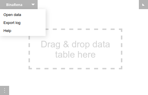
To open an input file, simply drag and drop it into the BinaRena interface, or click Open data in the context menu to open a file upload window.

Any supported file formats will be automatically parsed by the program, including:
- Data table (TSV with 2 or more columns, and with header)
- Mapping file (TSV with 2 columns, with or without header)
- Views (snapshots) of a dataset (JSON format, see details)
- Plain text listing members of a feature group (see details)
The first file opened in a fresh BinaRena window must be a data table. Then, during the analysis, you may append more files as needed by dragging and dropping them into the plot, or by clicking Load data/view in the context menu.
To work on multiple datasets simultaneously, just open multiple browser tabs.
A data table (tab-delimited file, or TSV) stores properties of contigs in an assembly. Here is an example.

Each row represents one contig. The first column must be unique contig identifiers. The remaining columns are arbitrary properties. Empty cells will be treated as missing values.
The first data table opened in BinaRena defines all contigs in a dataset. Later, you may append more tables or mapping files to the dataset (see above). They will be filtered to the intersection with the current contig list and merged into the current dataset.
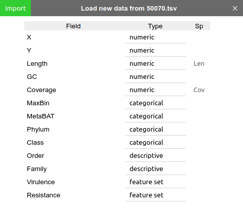
In loading a data table, BinaRena will prompt you to specify the data types of individual fields (columns):

Each field may be any of the following four types:
-
Numeric(
n): Such as length, coverage, GC%, etc. Can be either integers or floating point numbers. -
Categorical(
c): Such as taxonomic groups, external binning plans, etc. -
Feature set(
f): Features associated with each contig, such as genes. Should be written as comma-separated identifiers, such as "dnaK,rpoB,ftsZ". -
Descriptive(
d): Arbitrary free text, such as comments.
BinaRena will "guess" the most appropriate data type of each field based on the data. But you should still review, and correct any place where the program isn't smart enough.
One way to avoid manual review every time you open the same dataset, is to append a type code to a field name following a pipe (|), such as "genes|n" and "plasmid|c", in the raw TSV file.
Two properties are treated specially in BinaRena: length (bp) and coverage (x) of contigs, as they will be used to calculate bin abundance and to normalize bin summary metrics. They can be specified under the "Sp" column of the data import window ("Len" and "Cov"). BinaRena attempts to "guess" these two columns from the numeric columns based on their names (see how), but you still need to review, and correct if needed.
It is okay not to have either or both of these two columns in your dataset.
You can change these assignments later in the "Settings" window. This is useful when you explore a co-assembly with different coverage profiles of individual samples.
During the analysis, you can click Show data from the context menu to open a window to browse the current dataset. Alternatively, when one or more bins are selected, you can click the ◫ button in the bin table toolbar to browse the data of contigs within these bins.

One may click the "cross" button floating on each column head to delete this column from the dataset.
One may click Export in the table view to export the data table to a TSV file (see details).
See also scripts for generating input data.
Contact: Dr. Qiyun Zhu ([email protected]).