Tutorial

This tutorial provides a guide on preparing input data files for BinaRena.

In brief, BinaRena works with various properties of contigs in a metagenomic assembly. It is highly flexible to the types of properties it can handle. Some examples are length, GC%, coverage, k-mer frequency-based embedding, taxonomic classification, functional annotation, marker gene presence, and automatic binning results.

This tutorial walks you through a complete metagenomics workflow from scratch on a bioreactor metagenome. Popular software tools and protocols were chosen for individual steps. But you have the freedom to adopt and customize workflows that best suit your requirements.

• Note: This is not a tutorial of the BinaRena interface. If you already have your data files ready, please ignore this page and go straight to the live experience with BinaRena.

Please also check out:

• Guidelines on structuring input files, and a set of Python scripts to assist with input file preparation.
• Sample output files of this tutorial, and a Bash script containing all commands in the tutorial for reproducing the results.
• Another example dataset, which is a fully processed and combined table file. It is used in the live demo.

Software tools

Multiple bioinformatics programs will be used in this tutorial. If you are lucky, you will be able to install all of them using just one conda (or mamba) command:

conda create -n binarena-tutorial -c conda-forge -c bioconda megahit scikit-learn umap-learn bowtie2 samtools kraken2 prokka metabat2 checkm-genome
conda activate binarena-tutorial

Feel free to install the programs using your own methods or swap them with your favorite alternatives.

BinaRena scripts

BinaRena ships with multiple Python scripts to facilitate the preparation of input files. Download and extract these scripts:

wget https://github.com/qiyunlab/binarena/archive/refs/heads/master.zip
mkdir -p scripts && unzip -j master.zip binarena-master/scripts/*.py -d scripts
chmod +x scripts/*.py
rm master.zip

Sequencing data

In this tutorial we will use a bioreactor metagenome dataset which is part of the Earth Microbiome Project 500 (EMP500) (PRJEB42019) (Shaffer et al., 2022). This Illumina NovaSeq 6000 run (ERR5004366) contains 4M paired-end sequencing reads, totalling 590M bases. It is a very small dataset for demo purpose. To achieve optimal assembly and binning results you will need a higher sequencing depth.

for i in 1 2; do
  wget ftp://ftp.sra.ebi.ac.uk/vol1/fastq/ERR500/006/ERR5004366/ERR5004366_${i}.fastq.gz
done

The downloaded sequencing data are already post quality control. If not, you may use a program such as fastp, Trimmomatic or Cutadapt to perform quality control.

Metagenomic assembly

You may perform de novo assembly of the metagenome using choice of assemblers, such as MEGAHIT, SPAdes, IDBA-UD and Ray Meta. The following analysis uses MEGAHIT.

megahit -t 8 -1 ERR5004366_1.fastq.gz -2 ERR5004366_2.fastq.gz --min-contig-len 1000 -o megahit

This analysis uses 8 CPU cores to complete the task (same below). The output contig sequences must be at least 1000 bp (a common threshold for metagenome binning, but you may also try 500 or 2000).

Make a symbolic link to the output contig sequences. Now we can access them as contigs.fna.

ln -s megahit/final.contigs.fa contigs.fna

Basic contig metrics

The script sequence_basics.py obtains length, GC content, and coverage (if applicable) from contig sequences.

scripts/sequence_basics.py -i contigs.fna -a megahit -o basic.tsv

With the -a megahit parameter, the script automatically parses MEGAHIT contig titles (such as k141_1234 flag=1 multi=3.0000 len=1500) and extract the "pseudo" coverage value (here multi=3.0000).

• Note: This metric is roughly correlated with coverage and is good for a quick look of the data (see explanation). But the real coverage needs to be calculated by mapping reads against contig sequences, as discussed below.

k-mer signatures

The frequencies of k-mers are useful information for clustering and separating contigs. BinaRena provides two scripts: count_kmers.py for calculating k-mer frequencies in DNA sequences, and reduce_dimension.py for performing dimensionality reduction such that contigs can be visualized in the low-dimensional space (such as a 2D or 3D scatter plot).

scripts/count_kmers.py -i contigs.fna -k 5 | scripts/reduce_dimension.py --pca --tsne --umap -o k5

The above command counts k-mers with k=5 (a common value for metagenomic assemblies), then performs three dimensionality reduction methods: principal component analysis (PCA), t-distributed stochastic neighbor embedding (t-SNE) and uniform manifold approximation and projection (UMAP).

The output files k5.xxx.tsv (one per method) contain the coordinates of contigs in the two primary dimensions, which can be plotted as a 2D scatter plot.

Checkpoint

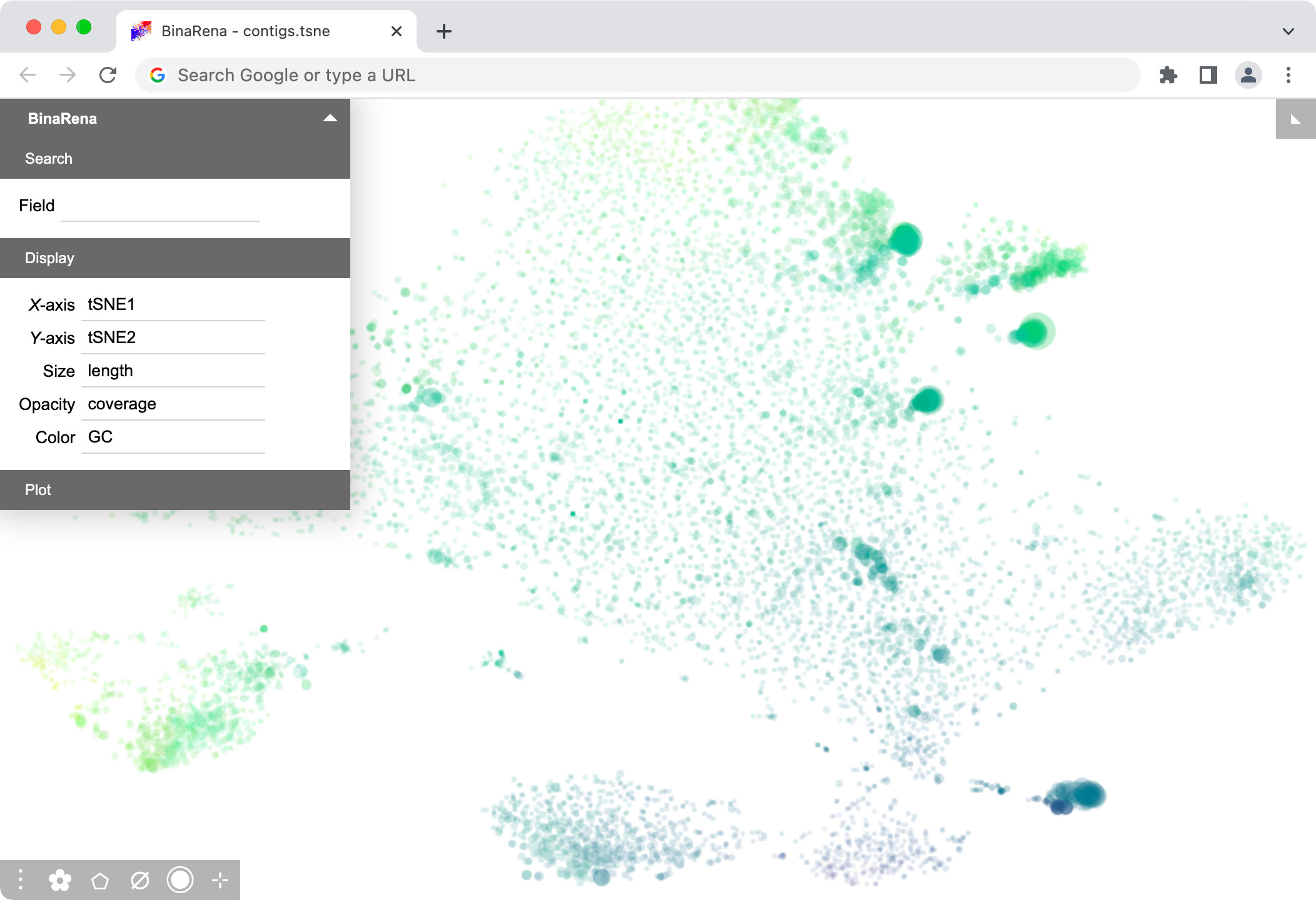
At this stage, if you are eager to see the outcome in BinaRena, you may already do so. Just sequentially drag and drop k5.tsne.tsv and basic.tsv into the BinaRena interface. Then set Size = length (cbrt), Opacity = coverage (sqrt), and Color = GC (none). A nice scatter plot should pop up!

Coverage calculation

The (mean) coverage (a.k.a. depth) of a contig is the average number of times each nucleotide is covered by a sequencing read.

Multiple tools and protocols can calculate contig coverages, such as BBMap, BEDTools and GATK. The following approach uses Bowtie2 with SAMtools.

First, generate a Bowtie2 index of the contig sequences. This index is used only once in this tutorial, but in a co-assembly setting you will map multiple datasets to the same index to assess per-sample contig abundances.

mkdir -p bt2idx && bowtie2-build --threads 8 contigs.fna bt2idx/contigs

Then map sequencing reads to the contigs using Bowtie2, and calculate contig coverages using SAMtools. Both analysis are streamlined in one command to avoid generating any intermediate files.

bowtie2 -p 8 -x bt2idx/contigs -1 ERR5004366_1.fastq.gz -2 ERR5004366_2.fastq.gz --no-unal | samtools sort -O bam > mapping.bam
samtools coverage mapping.bam > coverage.tsv

The output file coverage.tsv contains multiple columns, of which the 7th column meandepth is the said coverage measurement, whereas the coverage column is the percentage of the contig covered by any read (see details).

Using the following Bash trick, you can replace the previously generated "pseudo" coverage with the real coverage:

head -n1 basic.tsv > tmp.tsv
join -j1 -t$'\t' <(tail -n+2 basic.tsv | cut -f1-3 | sort -k1,1) <(tail -n+2 coverage.tsv | cut -f1,7 | sort -k1,1) | sort -V >> tmp.tsv
mv tmp.tsv basic.tsv

Taxonomic classification

The following approach uses Kraken2 to infer the taxonomic assignments of individual contigs. First, download a Kraken2 reference index:

wget https://genome-idx.s3.amazonaws.com/kraken/k2_standard_20230314.tar.gz
mkdir -p k2idx && tar xvf k2_standard_20230314.tar.gz -C k2idx
rm k2_standard_20230314.tar.gz

This is the "standard" index as of 2023-03-14. You may explore the official repository for other (and up-to-date) options that meet your needs.

Run Kraken2 to classify contig sequences:

kraken2 --db k2idx --threads 8 contigs.fna --output kraken2.output --report kraken2.report

The script kraken_to_table.py can convert classification results into a table of seven standard taxonomic ranks (from domain to species).

scripts/kraken_to_table.py -i kraken2.output -r kraken2.report -o taxonomy.tsv

Some other options of contig taxonomic classification are GTDB-Tk, CAT and Kajiu.

It should also be mentioned that the script lineage_to_table.py can convert lineage strings, which is the output format of software tools such as GTDB-Tk, into a table.

Functional annotation

The contig sequences can be annotated to inform the functional genes on them. Prokka is the classical workflow for annotating prokaryotic genomes (including metagenomes).

prokka contigs.fna --cpus 8 --outdir prokka --prefix contigs

This workflow generates multiple output files, of which contigs.gff is a GFF-formatted annotation file, listing predicted genes and their functional assignments in each contig.

The script gff_to_features.py extracts certain attributes (in this example: gene) from a GFF file and generates a mapping of contigs to the genes they contain:

scripts/gff_to_features.py -i prokka/contigs.gff -t gene -o gene.map

Some other annotation workflows are PGAP, Bakta and DeepFRI. You may also consider using database-specific tools, such as KofamKOALA (for KEGG) and eggNOG-mapper (for eggNOG).

Automatic binning

A variety of automatic binners, refiners and ensemblers are available on the shelf. BinaRena is not intended to replace automatic binning, but rather to complement it. With BinaRena, you may evaluate, compare and curate automatic binning results.

The following example demonstrates the use of a classical binner: MetaBAT2.

mkdir -p metabat2
jgi_summarize_bam_contig_depths --outputDepth metabat2/depth.txt mapping.bam
metabat2 -t 8 -i contigs.fna -a metabat2/depth.txt -o metabat2/bin -m 1500

The program outputs multiple FASTA files, each representing a bin, i.e., a set of contigs that presumably consitute a genome.

The following Bash trick generates a mapping of contigs to bins.

for i in metabat2/bin.*.fa; do
  bin=$(basename -s .fa $i)
  cat $i | grep ^'>' | cut -c2- | sed 's/$/\t'$bin'/' >> metabat2.map
done

We encourage you to explore the latest availability of automatic binning methods. The CAMI2 project (Meyer et al., 2022) provides a comprehensive evaluation of various binners, such as CONCOCT, MaxBin, SolidBin and Vamb. This may serve as an entry point for your exploration.

Bin quality evaluation

The quality of a bin can be evaluated by two metrics: completeness and contamination (redundancy), calculated based on the presence of single-copy marker genes specific to the lineage. CheckM is a classical method for this analysis. Typically, it operates on pre-defined bins, and the analysis is computationally intensive.

BinaRena provides a novel functionality, which calculates the completeness and contamination of any arbitrary group of contigs interactively and on the fly as you select them. It utilizes the CheckM results, but you just need to run CheckM once on the entire metagenome prior to running BinaRena.

• Please read more about this function here and here to understand what it does.

To start, you must specify which taxon you want to evaluate against. The following command uses domain Bacteria.

mkdir -p checkm/Bacteria
checkm taxonomy_wf domain Bacteria . checkm/Bacteria

The script checkm_marker_map.py converts the CheckM output into a contig-to-markers map:

scripts/checkm_marker_map.py checkm/Bacteria/storage/marker_gene_stats.tsv > checkm/Bacteria.map

The script checkm_marker_list.py converts the CheckM marker set definition into a marker list:

scripts/checkm_marker_list.py checkm/Bacteria/Bacteria.ms > checkm/Bacteria.lst

You may create these files for multiple taxa of interest. The command checkm taxon_list will show a list of them.

Finalization

Now that you have completed preparation of a comprehensive set of information for the contigs, you are ready to run BinaRena.

You may either combine the information into one table and load into BinaRena. There are multiple ways to do that. Or, you can simply drag and drop individual data files into the BinaRena interface. The program will combine the information for you.

Please sequentially drag and drop the following files, accept the default unless <= explicitly instructed, and click "Import".

• basic.tsv
• k5.pca.tsv
• k5.tsne.tsv
• k5.umap.tsv
• taxonomy.tsv
• gene.map <= Change data type to "feature set"
• metabat2.map
• checkm/Bacteria.map <= Change data type to "feature set"
• checkm/Bacteria.lst <= Change "for" to "Bacteria"

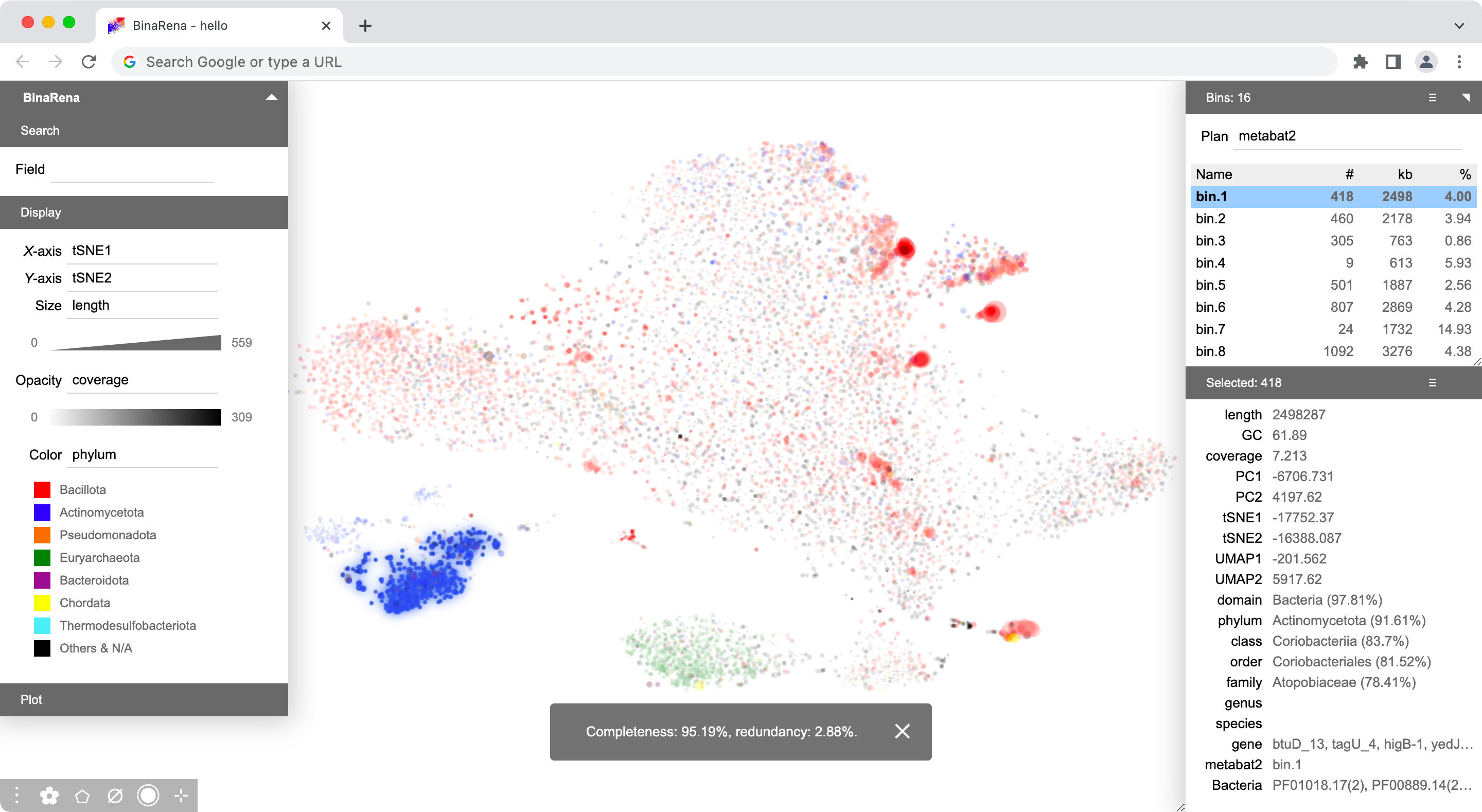
Then configure display items and their scaling methods in the "Display" panel:

• X-axis: tSNE1 (none)
• Y-axis: tSNE2 (none)
• Size: length (cbrt)
• Opacity: coverage (sqrt)
• Color: phylum

Here you go! Now it is your time to explore and play with your dataset!

You may right-click the plot and select Export data to generate a table file with all information combined (except for Bacteria.lst). Next time you can just drag and drop this table file, and the entire view will appear without manual attendance.