-
Notifications
You must be signed in to change notification settings - Fork 3
Post processing and use cases
RLM is a standalone application that processes a BAM file and returns output files containing methylation information and read-level metrics for and based on single reads. These output files can be used for downstream processing using common command line tools such as bedtools or UCSCtools and visualized in R. In the following, we describe the processing of an example file using RLM and simple potential steps to visualize the read-level information. We also provide a R Markdown script within this repository that creates global and - if desired - feature-wise summary statistics based on the RLM output.
Entropy, epipolymorphism, PDR and RTS can be visualized per 4-mer or CpG e.g. using UCSCtools:
cut -f 1,2,3,4 output_entropy.bed | sed '1d' | sort -k1,1 -k2,2n > entropy.bedgraph
bedGraphToBigWig entropy.bedgraph genome.chrom.sizes entropy.bw
Note: Entropy and epipolymorphism will be reported using the coordinates of the first CpG in a 4-mer.

Scores reported per CpG or 4-mer can be simply aggregated per feature e.g. using bedtools. The following example code shows how to calculate the mean entropy across a bed file with regions of interest (3 columns: chr, start, end):
bedtools intersect -a regions.bed -b output_entropy.bed -wa -wb | \
sort -k1,1 -k2,2n | \
bedtools groupby -i stdin -g 1,2,3 -c 7 -o mean > mean_entropy_regions.bed
The R script we provide requires R to be installed including the following packages:
knitrdata.tableGenomicRangesRColorBrewervioplotggplot2ggpubr
The script can be called the following way:
Rscript -e "rmarkdown::render('summarize_read_level_stats.Rmd',
params=list(
single_read_input_file = '/path/to/output_single_read_info.bed',
pdr_input_file = '/path/to/output_pdr.bed',
entropy_input_file = '/path/to/output_entropy.bed',
sample_name = 'my_sample',
feature_input_file = '/path/to/features.bed'),
output_file = 'my_output.pdf')"
The parameter feature_input_file is optional and if not provided, no feature-wise figures will be reported. If provided, it should be a bedgraph file of the following format: <chr> <start> <end> <feature_name> where <feature_name> should be the name of the feature type the region belongs to. For example, a feature file separating the genome into CpG islands (CGIs), CpG island shores (2kb upstream and downstream of a CGI), CpG island shelves (2kb upstream and downstream of the shores) and open water regions (the remaining parts) could look like the following:
chr1	0	3527624	OpenWater
chr1	3527624	3529624	CGIshelf
chr1	3529624	3531624	CGIshore
chr1	3531624	3531843	CGI
chr1	3531843	3533843	CGIshore
chr1	3533843	3535843	CGIshelf
chr1	3535843	3666619	OpenWater

...
The script will output a report containing basic statistics and figures of the single reads considered for the analysis, the reported PDR/RTS scores and the entropy/epipolymorphism scores. In the following, we will illustrate and explain the type of figures produced by the script using a WGBS sample of mouse epiblast (embryo tissue at embryonic day E6.5) as an example (GSM4075619).
First, the report summarizes the number of reads (total and discordant) that passed all filtering thresholds and were considered for the score calculations. Additionally, statistics regarding the number of CpGs per read (all and methylated), the transitions and the methylation per read are reported. The WGBS sample covers the complete mouse genome with high coverage. The majority of mammalian genomes are highly methylated while CpG-dense regions (CpG islands) usually remain free of methylation. This is reflected in the per read statistics were most reads genome-wide tend to have few CpGs but are highly methylated with few transitions between methylated and unmethylated CpGs.

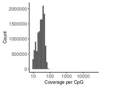
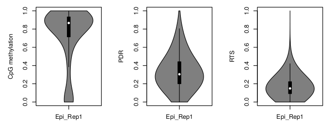
For PDR and RTS scores, the report summarizes the distribution of the coverage of reported CpGs. Additionally, violin plots visualizing the distribution of CpG methylation, PDR and RTS are provided. Some genomic regions artificially tend to get high amounts of reads during mapping which is why removing outlier CpGs with abnormally high coverage could be considered.
Generally, PDR is a very broad measure and will usually be higher than the RTS because a discordant read can have an arbitrary amount of transitions as long as there is at least one.
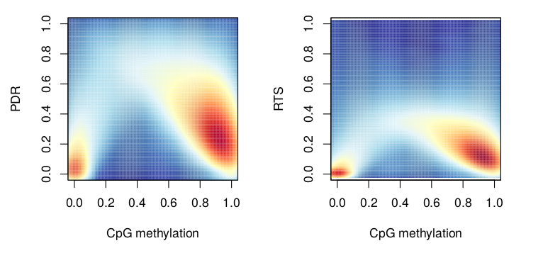
The relationship between methylation and PDR/RTS is summarized using smooth scatter plots where red refers to regions of high density while blue marks regions with low density. Regions with low and high DNA methylation in the genome will tend to have lower read level dynamics (i.e. low PDR or RTS) while intermediately methylated regions tend to have higher heterogeneity.
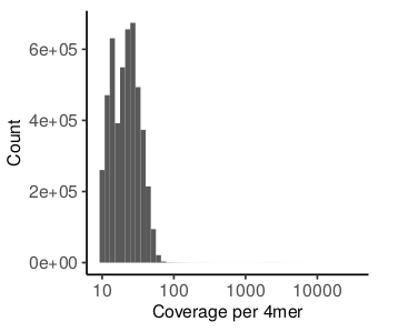
The report offers the same type of figures for entropy and epipolymoprhism scores. Importantly, here methylation and read level scores refer to a 4-mer of CpGs instead of a single CpG. The methylation per 4mer is calculated as the average methylation across all CpGs included. This average methylation will usually be lower compared to the CpG methylation reported PDR/RTS. For entropy and epipolymorphism, 4 CpGs in a row (4mer) are required to be present on a single read in contrast to the minimum of 3 CpGs that is required for PDR/RTS analysis. This biases the analysis towards CpG-rich regions such as CpG islands which tend to be unmethylated in mammalian genomes.

Again, regions with low and high DNA methylation in the genome will tend to have lower read level dynamics (i.e. low entropy or epipolymorphism) while intermediately methylated regions tend to have higher heterogeneity.

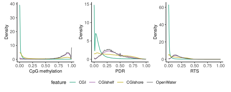
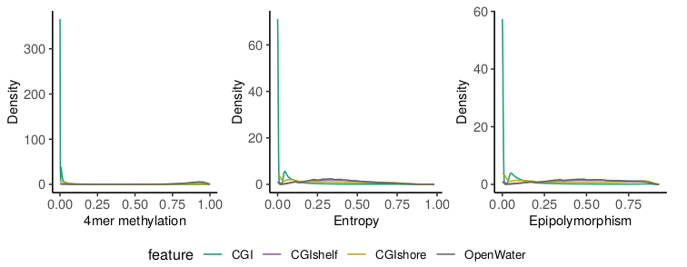
The script also offers the possibility to compare the distribution of methylation and read-level scores for different feature groups. This could be genomic regions such as CGIs or promoters but also differentially methylated regions (DMRs), imprinted regions, etc. As an example we compared CGIs with CGI shores, shelves and open water regions. As expected CGIs show low methylation levels which are accompanied by low heterogeneity based on read level scores. However, a group of CpGs/4-mers in CGIs shows higher read level scores indicating a different type of regulation of these regions. The lower the CpG density (i.e. going from CGIs to shores to shelves/open water) the higher the methylation accompanied by a rise in heterogeneity.
Read level analyses can be useful in a variety of applications where the pure methylation rates are not informative enough and specific interest regarding the underlying population dynamics exists. Scherer et al. provide a useful summary of potential use cases, applications and concepts. Generally, read level analysis might be useful for questions related to:
- Tissue heterogeneity
- Comparison of different conditions that are known to differ based on DNA methylation (this could be healthy and tumor tissue, wild-type and knockout contexts, etc.)
- Contamination of a cell population
- Methylation dynamics over time (such as in early mammalian embryonic development where DNA methylation is almost completely erased and re-established)
- Allele-specific methylation (i.e. imprinting)
- Comparing different features of interest such as DMRs or other genomic features not only based on average methylation differences but also regarding changes in underlying populations)