Getting Started with KnowledgeGraph
[This file is currently work in progress]
This Getting Started demonstrates how to fetch data from the Culture Knowledge Graph, how to collect meta-data from the German National Library, and how to combine and visualise the data in a basic network graph.
In addition, the Getting Started contains a universally transferable, beginner-friendly introduction to SPARQL (pronounced "sparkle"), a semantic query language used to access and retrieve data stored in graph-like RDF (Resource Description Framework) databases such as the Culture Knowledge Graph.
The Culture Knowledge Graph connects research data produced within the NFDI4Culture research landscape, improving the findability, accessibility, interoperability, and reusability of cultural heritage data. It brings together data from the Culture Research Information Graph and the Research Data Graph (for more information see this presentation). Data is provided as Linked Open Data and in part accessible via the NFDI4Culture Metadata RESTful API, but mainly via its SPARQL endpoint. The latter can be queried using the NFDIcore ontology as well as the NFDI4Culture ontology (cto) (which increasingly replaces the Culture Graph Interchange Format (CGIF)) in combination with further community standard ontologies.
From a content perspective, we will look at the letters of Ferdinand Gregorovius published by the German Historical Institute in Rome. The letters unveil Gregorovius' connections to his scientific peers in 19th century Europe and thus allow for a unique peek into the history of European science. The goal here will be to visualise Gregorovius' network by years. Of course, the preserved corpora only serves as an exemplary dataset to showcase one potential workflow that includes querying the Culture Knowledge Graph from within Facepager and linking the results with information from further databases.
To follow along, you will need to install the following software:
- Facepager (part 2)
- R and RStudio Desktop (part 3)
- Gephi (part 4)
Depending on your previous experience with the software, learning about Facepager's basic concepts will certainly make it easier follow.
DISCLAIMER: The Culture Knowledge Graph is work in progress. Currently, only a handful of datasets are accessible through its SPARQL endpoint using the NFDI4Culture Ontology. To get an up-to-date overview of the already integrated data feeds, please, see the Culture Knowledge Graph's public online dashboard. Furthermore, there will be user-friendly SPARQL Endpoint Explorer eventually. Yet, until published, a query containing only the url of a resource will result in a table describing all available metadata (see this example). The User-Policy and guidelines of the Culture Knowledge Graph are being worked on as well. For the time being we advise you to be mindful of potential query limits.
You have already learned how to pronounce SPARQL. Great! Yet, simply looking at a SPARQL query can be daunting. The whole structure and vocabulary, everything seems cryptic at first, not to mention the headache of writing a query from the ground up. No surprise, the syntax behind how data is stored was meant to to provide data with meaning in a machine-readable form. While SPARQL allows us to query all kinds of databases, it still follows a syntax that was tailored to machines not humans. In the following sections, we will break down the logic behind SPARQL step-by-step so you will eventually be able to read its syntax just as easily as you read this way too long introduction.
What then are RDF Triples, did you not want to teach me about SPARQL, you ask. Well, yes, but to do so, let's first take one step back: Imagine you had an appointment with the authorities but not only is every door labelled in a different language which makes it hard for you to find the correct room, you also have to speak different languages when applying for a passport versus registering a new place of residence. That would not be particularly efficient, would it? The same applies to huge databases where lots of different information are stored. To prevent users from having to learn a new language every time they wanted to retrieve or store data a common standard for communicating with database was needed. Now, the Resource Description Framework, or RDF for short, is just that: a standard model for data interchange on the web. It has a simple syntax that is based on triples consisting of a subject, a predicate, and an object (e.g. "Susan has age 42"). Several such triples can be formalised as networks or knowledge graphs. SPARQL, on the other hand, is the semantic query language that is commonly used to query data from RDF's triple stores. Because RDF dictates data to be stored in triples, we can retrieve it using triple statements as well. Thus, all SPARQL statements are made up of the same three elements: a subject, a predicate and an object. A person's age, for instance, can be formulated as follows: Susan (subject) has age (predicate) 42 (object). In principle, all dates can be formalised as such triples.
?sub ?pred ?obj .

Susan has age 42 .
The RDF was developed to bring various different data models down to the lowest common denominator, and yet it does not define the format in which data is stored. Formats range from JSON-LD, XML/RDF to text formats such as Turtle. Often several formats are available to choose from, as RDF makes them interchangeable. For a detailed introduction to RDF see, Jünger and Gärtner (2023) Computational Methods for the Social Sciences and Humanities (Chapter 3.7).
Many free online databases let users execute queries via so-called SPARQL endpoints that are implemented in RDF databases. These endpoints act as an interface between the user and the underlying RDF data, enabling queries to be submitted over the web. Well-known SPARQL endpoints are provided by DBpedia or Wikidata. The NFDI4Culture also provides a public SPARQL endpoint. You will get to use them soon!
Let's now turn to the heart of it all. Consider the following SPARQL query:
SPARQL queries, as already established, allow you to search and query data from RDF formatted databases or knowledge graphs. While at its core, a SPARQL query consists of triple statements, it features all of the following basic elements:
- PREFIX: Defines prefixes for namespaces to, one, improve the readability of queries and, two, tell what data can be queried using which vocabulary. Do not worry about it for now. We will turn to Namespaces and Vocabularies shortly.
- SELECT: Determines what results will be returned from the query.
-
WHERE: Defines the patterns that are searched for in the RDF graph. Remember all data can be found using triples and here is where to put them. Because we want to request information, we work with placeholders or variables that are embedded in the triple structure. Variables can be recognised by the
?in front of them. - OPTIONAL: Allows optional patterns that do not necessarily have to be present in the graph. This is especially helpful, if you query for data that is not certainly available.
- FILTER: Used to filter results based on predefined conditions.
-
SORTING PARAMETERS: Use
LIMIT,GROUP BYorORDER BYto limit or sort the returned results. Without an explicit instruction, the results are returned in the order in which they are processed by the RDF database or the SPARQL endpoint.
For starters, we can create a simple SPARQL query by asking for an unspecified triple of subject, predicate, and object. Remember to set a low LIMIT. The less specific your query, the higher the chance that an astronomical number of results will bring the query to its knees. Let's try to query the DBpedia SPARQL Endpoint. Simply, paste the query below and hit Execute Query.
PREFIX rdf: <http://www.w3.org/1999/02/22-rdf-syntax-ns#>
PREFIX rdfs: <http://www.w3.org/2000/01/rdf-schema#>

SELECT ?sub ?pred ?obj
WHERE {
  ?sub ?pred ?obj .
} LIMIT 10
This pattern will match any triple in the RDF graph, effectively retrieving all triples at once (limited to the first 10 results). Congratulations! You have successfully created your first SPARQL query. Now, let's try something a little more ... insightful that we can actually make sense of. Let's catch the first ten persons' names, stored in DBpedia. Again, paste the query below and hit Execute Query.
PREFIX foaf: <http://xmlns.com/foaf/0.1/>

SELECT ?name
WHERE {

?person foaf:name ?name .

} LIMIT 10
That worked! But notice how the returned names do not seem to belong to humans but to all kinds of entities? That's because ?personis a variable with no meaning. To fetch the names of actual persons, we have to incorporate a triple statement that tells the database that we are only looking for entries with the attribute person. Notice, how by using a ; we separated multiple predicates that refer to the same subject:
PREFIX foaf: <http://xmlns.com/foaf/0.1/>

SELECT ?name
WHERE {

?entity a foaf:Person ;
		  foaf:name ?name .

} LIMIT 10
Far better! Using SPARQL, we used the first triple to tell that our variable ?entity (subject) is a (predicate) foaf:Person(object). that means an entity that is defined as a person through the FOAF (Friend of a Friend) namespace, which provides terms for describing people. Note, how we had to define the prefix first! Using ; we then added another triple referring to the same subject ?entity. This time, however, we got the predicate (foaf:name) from FOAF which points to the entity's name. Lastly, we store the resulting object in another variable (?name). As we only selected ?nameto be returned, that is all we see. Try to select ?personas well and see what happens.
Literally, the query can be read aloud as follows: ?entityis a person (as defined by FOAF) and has the name ?name.
Now that you know the basic syntax, let's talk about prefixes, namespaces, and vocabularies. You already encountered a common namespace, namely Friends of a Friend. A namespace defines the vocabulary used to clearly label the elements of a triple. Vocabularies contain defined expressions for certain categories such as names or birthdays and all kinds of other information. FOAF, for example, stores predicates such as names, addresses or acquaintances in a standardised manner. Other common vocabularies come from schema.org or DBPedia itself. Within a SPARQL query, we call this vocabularies by setting a Prefix. Prefixes are abbreviations of their namespaces' full URIs:
PREFIX foaf: <http://xmlns.com/foaf/0.1/>
PREFIX schema: <http://schema.org/>
PREFIX dbo: <http://dbpedia.org/ontology/>
PREFIX dbp: <http://dbpedia.org/property/>
A collection of related terms, for example that people have a name or a date of birth, or that a book has a title and a publishing year is called an ontology. Ontologies are formalised with languages such as the Web Ontology Language (OWL).
Now that you have learned about the fundamental basics of SPARQL, you are ready to take a look at the query that allows us to experience Ferdinand Gregorovius' connections to his scientific peers in 19th century Europe. The information we are looking for are stored in the Culture Knowledge Graph provided by NFDI4Culture. You can run the following query yourself at the NFDI4Culture's dedicated public SPARQL endpoint.
# Start by defining all prefixes needed to formulate the query
PREFIX cto: <https://nfdi4culture.de/ontology#>
PREFIX schema: <http://schema.org/>
PREFIX rdf: <http://www.w3.org/1999/02/22-rdf-syntax-ns#>
PREFIX rdfs: <http://www.w3.org/2000/01/rdf-schema#>
PREFIX n4c: <https://nfdi4culture.de/id/>

# Select the variables of interest
SELECT ?letter ?letterLabel ?date ?gnd_id
WHERE {

# Fetches all items from the 'Letters from the Digital Edition Ferdinand Gregorovius'
# dataset. All items are letters.
n4c:E5378 schema:dataFeedElement/schema:item ?letter .

# For each letter retrieve its label..
?letter rdfs:label ?letterLabel ;
		# ..its creation date..
		cto:creationDate ?date ;
		# ..and the URLs pointing to the GND entry of all persons mentioned within.
		cto:gnd ?gnd_url .

# Only return letters written in 1951.
FILTER(YEAR(?date) = 1951).

# Extracting the GND IDs from the GND URLs for further processing
BIND(REPLACE(STR(?gnd_url), ".*://.*/(.*?)", "$1") AS ?gnd_id)

}-
PREFIXES: The data we want to retrieve hides behind a number of different vocabularies. Note how the CultureKnowledgeGraph is based on its on ontologies
ctoandn4calongside common vocabularies. If you are wondering how the vocabulary of a particular ontology is structured, it is usually worth looking directly through the documentation of a namespace. In order to understand which ontologies a graph database is based on in the first place, the documentation of the graph helps. Albeit unrelated to this query, the graph description provided by the team behind SemOpenAlex is comprehensive, beginner-friendly example of this. -
SELECT: We are interested in the all letters from a specific year (
?letter), its title (?letterLabel), date (?date), and the GND ID of all persons mentioned in the letter (?gnd_id). -
WHERE: To make the context of the individual triples easier to understand, we have commented on the query line by line. Comments are indicated by
#. - OPTIONAL: Allows optional patterns that do not necessarily have to be present in the graph. This is especially helpful, if you query for data that is not certainly available.
- FILTER: The filter is at the heart of our query. We use it to fetch all letters from a specific year, in this case 1951.
- SORTING PARAMETERS: We did not limit of sort the list of results, because we are interested in all results and will sort them later on. We do know, however, that the results won't exceed an unreasonable number and won't occupy the endpoint's full capacity.
You might, at least, want to read through Part 2 of this Getting-Started to better understand the goal of this query.
Facepager supports querying graph databases using SPARQL via the Generic module at the moment. We are currently working on a dedicated SPARQL module that will allow users to build and test queries more practically without having to leave the software. However, there is one central peculiarity that always needs to be taken into account when issuing a SPARQL query using Facepager. Facepager marks seed node placeholders such as the object ID with arrow heads: <Object ID>. As you may have noticed, usually, the namespaces in SPARQL queries are also labelled with arrow heads. In order for Facepager to resolve a SPARQL query correctly, every arrow head must be escaped \<LINK TO ONTOLOGY\>, except of course the ones marking the <Object ID>. For an illustration, see the same SPARQL query as before, optimised for Facepager.
PREFIX cto: \<https://nfdi4culture.de/ontology#\>
PREFIX schema: \<http://schema.org/\>
PREFIX rdf: \<http://www.w3.org/1999/02/22-rdf-syntax-ns#\>
PREFIX rdfs: \<http://www.w3.org/2000/01/rdf-schema#\>
PREFIX n4c: \<https://nfdi4culture.de/id/\>

SELECT ?letter ?letterLabel ?date ?gnd_id
WHERE {

n4c:E5378 schema:dataFeedElement/schema:item ?letter .

?letter rdfs:label ?letterLabel ;
		cto:creationDate ?date ;
		cto:gnd ?gnd_url .

FILTER(YEAR(?date) = <Object ID>).

BIND(REPLACE(STR(?gnd_url), ".*://.*/(.*?)", "$1") AS ?gnd_id)

}Making an effort to learn the basics of SPARQL and its syntax will allow you to literally understand any graph database query and, more crucially, will let you write your own queries to fetch data from all kinds of public knowledge graphs. A great resources to learn more about SPARQL and some of its advanced syntax quirks is Wikidata's introduction to SPARQL.
We begin by fetching detailed information about the letters of Ferdinand Gregorovius from a specific year(s) stored in the Culture Knowledge Graph. The benefit of using Facepager to issue the query instead of the online SPARQL endpoint will reveal itself once we want to complement our initial fetch with data from other databases. Let's dive in:
- Create a database: Click New Database in the Menu Bar of Facepager to create a blank database. Save it in a directory of your choice.
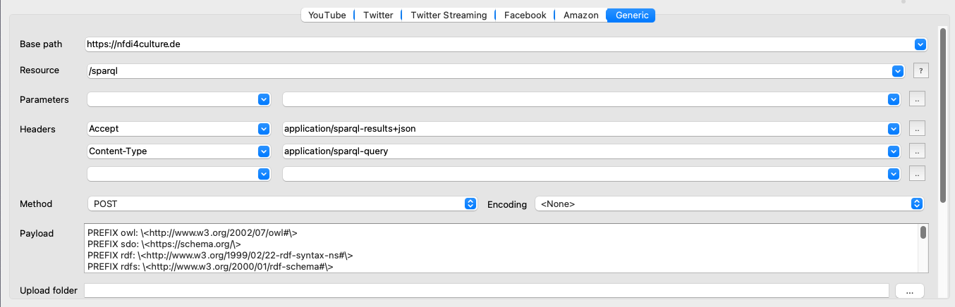
- Setup the Generic module: From the Presets tab in the Menu Bar select and Apply the NFDI4Culture preset "1 Get GND IDs of Ferdinand Gregorovius' letter addressees". The Generic module in the Query Setup will refresh instantly. Notice that the base and resource paths are now set to call the SPARQL endpoint of NFDI4Culture. Additionally, two Headers have been placed. Accept specifies the data format returned by our query. We want the results to be returned in JSON-format. Content-Type prepares the query by requesting an unencoded SPARQL query string. As we will query via POST directly, it is crucial to set the Method to POST. For a more detailed explanation of all adjustments, check the SPARQL chapter from the Triply API documentation. At the heart of our data collection lies the SPARQL query that we have developed in part 1 of this tutorial. When the presets gets applied, the prepared query loads directly into the Payload box. Again note, that is has been optimised for Facepager by escaping all common arrow heads.
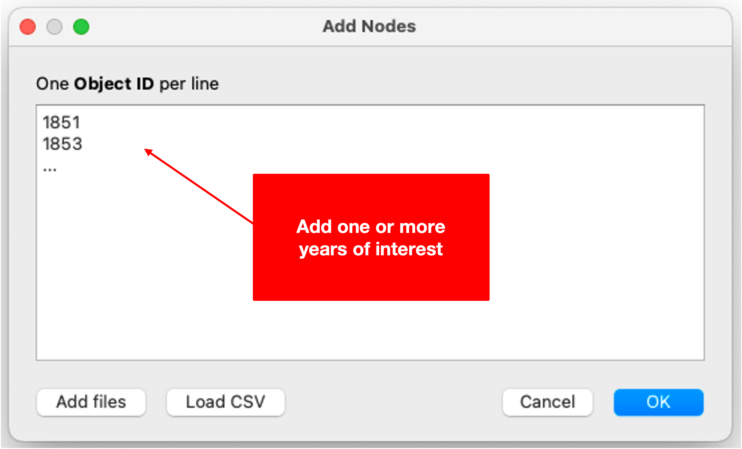
- Add nodes: Before fetching data, you will need to provide one or more seed nodes which will fill in the placeholder mentioned above during the actual request. To do so, select Add Nodes in the Menu Bar. In the open dialogue box enter one or more years (e.g. 1851, 1853, etc.). If you have a closer look at the SPARQL query (see part 1), you will find that your seed nodes will fill in a placeholder within a filter restricting the results to the years specified. Include as many nodes (years) as are of interest to you.
- Fetch data: Select one or more seed nodes, then hit Fetch Data at the bottom of the Query Setup. Facepager will now fetch data based on your setup. Once finished, you can inspect the data by expanding your seed node or clicking Expand nodes in the Menu Bar. For more detail, select a child node and review the raw data displayed in the Data View to the right. The information here can be a little messy. To get a comprehensive overview of only the data interesting to you, play around with the Column Setup to define what information will be displayed in the Nodes View.

Because we are interested in the addressees of Ferdinand Gregorovius, what we want to be displayed is the date of any given letter from the specified year, the letter's label, and the names of all persons addressed or mentioned by Gregorovius. However, these names are glaringly missing. They are not contained within the data we fetched. Instead, what we do find are GND IDs of Gregorovius' relations. GND IDs refer to the "Gemeinsame Normdatei" (Integrated Authority File) ID. It is used in Germany primarily for the unique distinction of entities in library catalogs and allows to manage and link bibliographic records. Fortunately for us, the German National Library provides Entity-Fact sheets which we can use to quickly translate the GND IDs stored in the Culture Knowledge Graph by applying a second preset. This is where Facepager's strong suit comes into play.
- Apply second preset: To do so, from the Presets tab in the Menu Bar select and Apply the NFDI4Culture preset "2 Translate GND ID to a person's name". The Generic module in the Query Setup will refresh instantly. Now, the base and resource paths are set to call the Entity Facts API of the German National Library (DNB). Further, a new placeholder is introduced as a parameter. The key parameter specifies what information will be returned. The preset at hand only asks for the preferredName associated with a GND ID. See this overview to get an idea of the data provided by the Entity Facts API. Please, mind the German National Library's [Terms of Use](https://www.dnb.de/EN/Professionell/Metadatendienste/Datenbezug/geschaeftsmodell.html).

- Add nodes: Before fetching data, usually you would have to provide one or more seed nodes which would then fill in the placeholder mentioned above during the actual request. However, this time this is not to be done manually. Notice that the Object IDs of all child nodes from our first data collection already match the GND IDs we are interested in.

- Fetch data (again): Therefore, simply select all child nodes instead and Fetch Data again. Facepager will fetch data based on your setup once more. Once finished, you can inspect the data by expanding your child node or clicking Expand nodes in the Menu Bar. For more detail, select one of the new child nodes and review the raw data displayed in the Data View to the right. Again, the information here can be overwhelming. For now, we are only interested in the preferred name of a person. The preset has already adjusted the Column Setup accordingly. You have now successfully translated the GND IDs into more meaningful names. Our dataset is complete.
- Export data: Expand all nodes and select the ones you want to export. Hit Export Data to get a CSV-file. Notice the options provided by the export dialogue. You can open CSV files with Excel or any statistics software you like.
If you want to prepare and clean the data to eventually visualise them in a network graph, continue to follow the last two sections of this Getting-Started.
If you wish to continue by visualising the data you just collected, the next step is all about data preparation using RStudio. The R script below serves as a jump-start and instantly creates a nodes list and an edges list both needed for the network analysis later on.
- Begin by creating a new RStudio project.
- Move the CSV file (ckg_gregorovius.csv) into the project directory.
- Create a new R script, paste the following code, then run the script to produce two new CSV files containing nodes and edges. They will be saved in your project directory. Make sure to set the working directory to the source file location via the Session tab in the menu bar.
# load packages and data
library(tidyverse)

data <- read_csv2("ckg_gregorovius.csv")

# prepare data
# - convert parent_id from string to numeric to enable left_join (as.numeric)
data$parent_id <- as.numeric(data$parent_id)

# - filter out irrelevant rows  (filter)
# - merge rows where id and parent_id match across rows (left_join)
# - combine values, rename & select relevant columns (mutate & select)
# - remove redundant rows by dropping NAs (drop_na)
data <- data %>%
  filter(object_type == "data") %>%
  left_join(data, by = c("id" = "parent_id"), suffix = c("", ".y")) %>%
  mutate(
    year = year(date.value),
    addressee = coalesce(preferredName, preferredName.y)
    ) %>%
  select(
    id,
    parent_id,
    gnd=object_id,
    year,
    addressee,
    letter=letterLabel.value
    ) %>%
  drop_na()

# edges
# - join parent row to every row  (left_join)
# - select and rename columns  (select)
# - remove duplicates  (distinct)
edges <- data %>%
  left_join(data,by="letter") %>%
  filter(gnd.x != gnd.y) %>%
  select(source=gnd.x,target=gnd.y) %>%
  distinct() %>%
  na.omit()

# nodes
# - select and rename columns (select)
# - remove duplicates (distinct), omit if frequency is of relevance
nodes <- data %>%
  select(ID=gnd,Label=addressee, year) %>%
  distinct()

# save nodes and edges for Gephi
write_csv2(edges,"gregorovius_edges.csv",na = "")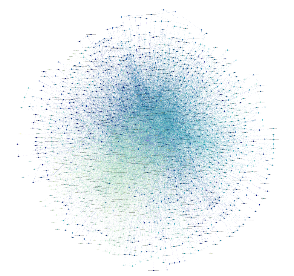
write_csv2(nodes,"gregorovius_nodes.csv",na = "")You are now ready to visualise the data in Gephi and get an intuitive idea of Ferdinand Gregorovius' social network of the 19th century. Gephi is of course not your only option. R and RStudio, for example, let you build network graphs as well.
- Import data: Find the Import spreadsheet button in the Data Laboratory tab to first load the nodes list and then the edges list. When navigating the dialogue box, make sure that you import the nodes list as a Nodes table and the edges list as an Edges table. Select Append to existing workspace at the end of the import.
- Organise network: Head back to the Overview tab to see your nodes distributed randomly in a dense cloud. Run the layout algorithm Fruchterman Reingold to kick-start your network visualisation. In this layout, the more frequent nodes are connected the closer they are positioned closer to each other. Take some time to play around with settings. Further exploration of the network might be enable by altering the colour or size of nodes in the Appearance section or by applying time-based filters.
- Export network graph: Select the Preview tab to export your network graph either as SVG, PDF, or PNG. Here, you will also find some additional options to finalise the appearance of your graph.

There is a wealth of resources available online to get a more profound idea of the available features in Gephi. Start by looking up tutorials on YouTube about network visualisations as well as analyses and check out briatte's Awesome Network Analysis resource list on GitHub. Or, if German does not scare you off, have a look at Jünger and Gärtner's (2023) open-access introduction to Computational Methods for the Social Sciences and Humanities (Chapter 3 focusses on data formats, Chapter 10 on network analyses).
- If network graphs intrigue you, look into our Getting Started with YouTube Networks or Getting Started with Wikidata to gain more inspiration of the analyses possible with Facepager.
- In Facepager itself you will find further presets that allow you to call up various freely accessible graph databases using SPARQL. Simply, check out our Preset category "Knowledge Graph" to quickly get started.
- For an overview of what other data can be fetched using Facepager, browse through our diverse Getting Started series. Learn, for example, how to obtain detailed information about scholarly works stored in OpenAlex' free and open online repository of the world's research system.