User Guide
This guide provides more information on how to use pyBAR.
PyBAR is built on top of the Basil framework. Basil is providing FPGA firmware modules and drivers.
The PyBAR project folder contains several subfolders:
- examples: several examples on the usage of pyBAR
- firmware: FPGA projects for MIO, MIO3, MMC3 and SEABAS2
- pybar: folder containing the host software
The pybar folder contains the host software and binary files for programming the hardware:
- analysis: analysis and plotting library (C++ and python code)
- config: default FE-I4 configuration files (deprecated, default config is taken from fei4_defines.py)
-
daq:
- fei4_raw_data.py: storing FE-I4 raw data to data output file. Contains connector to online monitor.
- fei4_record.py: prints and decode FE-I4 raw data (for debugging)
- fifo_readout.py: FIFO readout thread (using Basil)
- readout_utils.py: converting and selecting FE-I4 raw data (for debugging)
-
fei4:
- fei4_defines_.py: FE-I4 commands, and initial configuration parameters
- register.py: generating FE-I4 commands
- register_utils.py: sending commands (using Basil) and helper functions
- scans: pyBAR run scripts (see below for more details)
- testing: several tests to test program code for errors and a simulation of the readout system with FE-I4
-
utils:
- utils.py: helper functions
- configuration.yaml: main configuration file (see below for more details)
- dut_configuration_mio.yaml: Basil initialization configuration for MIO + Single Chip Adapter Card/Burn-in Card (see below for more details)
- dut_configuration_mio_gpac.yaml: Basil initialization configuration for MIO + GPAC (see below for more details)
- dut_configuration_seabas2.yaml: Basil initialization configuration for SEABAS2 (see below for more details)
- dut_mio.yaml: Basil configuration file for MIO + Single Chip Adapter Card/Burn-in Card (see below for more details)
- dut_mio_gpac.yaml: Basil configuration file for MIO + GPAC (see below for more details)
- dut_seabas2.yaml: Basil configuration file for SEABAS2 (see below for more details)
- fei4_run_base: abstract run script for pyBAR doing all the initialization and excution of the three main scan functions configure(), scan(), analyze()
- online_monitor.py: the online monitor
- run_manager.py: basic run manager and abstract run script (very generic, not FE-I4 specific)
PyBAR comes with different FPGA bit files, which are providing support for different hardware platforms and adapter cards. The bit files are located in the pybar folder.
- mio.bit: MIO support with Single Chip Card or Burn-in Card (Quad Module Adapter Card)
- mio_gpac.bit: MIO support with GPAC (General Purpose Analog Card)
- seabas2.bit: SEABAS2 support
Note: The FPGA projects are located in the firmware folder.
PyBAR has several configuration files that helps to set up your test system:
-
configuration.yaml:
This is the main configuration file. By default, the pyBAR run scripts are using the settings from the configuration.yaml file in pybar folder. The configuration.yaml contains all the necesary information about the hardware setup, the FEI4 flavor and configuration, and the data output folder.
The data output folder, if not existing, will be created during the first run. The data output folder is given by themodule_idparameter inside the configuration.yaml file. It contains the raw data generated during a run, and analyzed data, PDF output files, and the FE-I4 configuration files, which are generated at the end of each run. In addition one can find the run.cfg containing information about each run (exit status, run name, start and stop time), and the crash.log containing traceback information if the exit status was “CRASHED”.
It is also possible to add run configuration for each run script that deviates from the default run configurtion. Examples are given inside the configuration.yaml file. -
dut_mio.yaml, dut_mio_gpac.yaml, dut_seabas2.yaml:
Basil configuration file containing all the necessary information about the DUT (hardware setup). -
dut_configuration_mio.yaml, dut_configuration_mio_gpac.yaml, dut_configuration_seabas2.yaml:
Basil initialization configuration with initialization parameters that will be used during initialization of the DUT. Initialization parameters can be FPGA firmware file, register values for firmware modules.
The standard config parameters are loaded from the fei4_defines.py (equivalent configuration files are located here).
An initial set of configuration files are generated during the first run and stored inside the data output folder. The flavor of the initial configuration file is given by the fe_flavor parameter inside configuration.yaml file. A configuration is stored after each run, whether or not the configuration has changed.
The FE-I4 configuration is splitted up into several files. The configs subfolder contains the main configuration files. They contain the global configuration, chip parameters, calibration parameters and the paths to the pixel configurations.
The masks subfolder contains all masks (C_high, C_low, Enable, DigInj, Imon). The column number is given on top and the row number on the left:
###  1     6     11    16     21    26     31    36     41    46     51    56     61    66     71    76
  1  11111-11111  11111-11111  11111-11111  11111-11111  11111-11111  11111-11111  11111-11111  11111-11111
  2  11111-11111  11111-11111  11111-11111  11111-11111  11111-11111  11111-11111  11111-11111  11111-11111
  3  11111-11111  11111-11111  11111-11111  11111-11111  11111-11111  11111-11111  11111-11111  11111-11111
  4  11111-11111  11111-11111  11111-11111  11111-11111  11111-11111  11111-11111  11111-11111  11111-11111

  ...
The TDAC and FDAC settings are placed in the tdacs and fdacs subfolder, respectively. To make the content fit on a computer screen, one line represents only the half of a FE column. The indices on the left represents the row number and a stands for columns 1-40 and b for columns 41-80:
###    1  2  3  4  5  6  7  8  9 10   11 12 13 14 15 16 17 18 19 20   21 22 23 24 25 26 27 28 29 30   31 32 33 34 35 36 37 38 39 40
###   41 42 43 44 45 46 47 48 49 50   51 52 53 54 55 56 57 58 59 60   61 62 63 64 65 66 67 68 69 70   71 72 73 74 75 76 77 78 79 80
  1a   8  8  8  8  8  8  8  8  8  8    8  8  8  8  8  8  8  8  8  8    8  8  8  8  8  8  8  8  8  8    8  8  8  8  8  8  8  8  8  8
  1b   8  8  8  8  8  8  8  8  8  8    8  8  8  8  8  8  8  8  8  8    8  8  8  8  8  8  8  8  8  8    8  8  8  8  8  8  8  8  8  8
  2a   8  8  8  8  8  8  8  8  8  8    8  8  8  8  8  8  8  8  8  8    8  8  8  8  8  8  8  8  8  8    8  8  8  8  8  8  8  8  8  8
  2b   8  8  8  8  8  8  8  8  8  8    8  8  8  8  8  8  8  8  8  8    8  8  8  8  8  8  8  8  8  8    8  8  8  8  8  8  8  8  8  8

  ...
Once, the data output path is filled with first data, the configuration for the FE-I4 can be specified. There are different methods how to do it which involve changing the fe_configuration parameter in the configuration.yaml:
- Leave it blank. The configuration with the highest run number and run staus FINISHED will be taken from the data output folder.
- Select configuration by run number:
fe_configuration : 42 - Specify configuration file by full or relative path:
fe_configuration : ../42_scan_analog.cfg - Specify configuration from data output file (HDF5 file) by full or relative path:
fe_configuration : ../42_scan_analog.h5
Note:
- The configuration files (.cfg) are created after the data analysis at the very end of a run. They may contain modifications made to the FE-I4 configuration. In contrast, the data output files (.h5) contain the initial FE-I4 configuration at the very beginning of a run (e.g. tuning results are thus not stored in the h5 file).
- The file format is similar to the RCE system configuration files.
The data files are using the HDF5 file format (.h5). HDF5 is designed to store and organize large amounts of data. The data are organized in nodes and leafs. PyTables is a package for managing HDF5 files. It is built on top of the HDF5 library and is providing additional features like fast compression via the BLOSC filter and a table data structure.
One can distinguish between data files at two different stages:
- data output files containing the data generated during a run (raw data, meta data, parameter data, configuration data)
- interpreted data files containing interpreted/analyzed data (histograms, hit and cluster tables)
The interpreted data is usually generated at the end of a run during the analyze step.
The data output file is created at the beginning of a scan and data is added at every readout. The file contains four different nodes: the FE-I4 raw data, the meta data, the configuration, and the scan parameter data (optional).
- Raw data
The raw data contains all FE words + FPGA trigger words + FPGA TDC words in an one dimensional array.
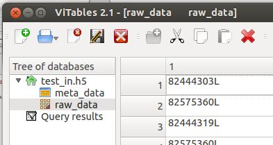
Every word is a 32-bit unsigned int. The format is: 82444303 = 0 000 0100 1110 1010 0000 0000 0000 1111
If the first bold bit is 1 the word is a trigger word followed by a trigger number. If it is 0 the following bits indicate the FE number. This number is usually 5 when you use the single chip adapter card. With other adapter cards (e.g. burn-in card) this number identifies the different FE connected to it. The remaining 24-bits hold the FE word. For more information (e.g. TDC word) please look here.
- Meta data
The meta data stores read out related infos:

One row is added for every read out. It contains the word index at the first / last+1 word of the read out and the total numbers of words. To allow time based analysis it also has a timestamp and an error code indicating read out errors (like out of sync). The error code is not used so far.
- Configuration data
All configuration parameters needed to be able to repeat the scan are stored here in different nodes.
This includes the Front-End configration, the specific run configuration etc.
- Parameter Data
In the parameter table the parameters that are changed during a scan is monitored (e.g. PlsrDAC setting during a threshold scan). At every readout the acutal parameter settings is added to the table. One column is reserved for one parameter.
The raw data is interpreted, analysed and plotted with the raw data converter class. The output HDF5 file can hold hit data, cluster data, meta data and histograms at different HDF5 notes.
-
Hit data
The hit data table stores the information for every hit.

The columns are:- event_number: The absolute event number. Only events with hits appear here.
- trigger_number: The TLU trigger number. If no TLU is used the trigger number is always 0.
- relative_BCID: The relative BCID is the number of data headers of one event when the hit occured.
- LVL1ID: The LVL1ID is the internal LVL1 trigger counter value of the FE.
- column: the column position of the hit
- row: the row position of the hit
- tot: the tot code of the hit
- BCID: the absolute BCID value
- TDC: the TDC value. If TDC was not used this values is always 0.
- TDC_time_stamp: the TDC time stamp value. If not used it is always 255.
- trigger_status: the trigger status of the event where the hit occured. The trigger status error code is a sum of the different binary coded trigger error codes that occured during the event. Please take a look at the histogram section for the error code explanation.
- service_record: the service records that occured in the event of the hit. The service record code is a sum of the different binary coded service records that occured during the event.
- event_status: the status of the event of the hit. The event error code is a sum of the different binary coded event error codes that occured during the event. Please take a look at the histogram section for the error code explanation.
-
Meta data
There are two output tables for meta data. The table called MetaData is a copy of the input meta table (see Scan data section above), but has event numbers instead of raw data word indices and additional scan parameter columns for each scan parameter.
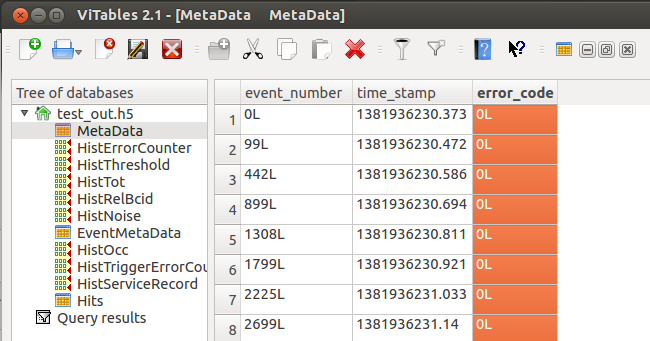
The table EventMetaData stores the start and stop raw data word indices for each event. This table is usually not created and only needed for in depth raw data analysis. It can act as a dictionary to get the connection between event number and raw data words of the event.

-
Hit Histograms
During raw data interpretation a lot of different histograms can be created on the fly. Usually single hit information is less interesting while histogram data provides sufficient information. The most common histograms are listed below, including there plotting representation created by the pyBAR plotting module:- HistOcc: The occupancy histogram stores the FE hits for each scan parameter in a three dimensional map. The first two dimensions reflect the pixel alignment (col x row) and the third dimension is the scan parameter.
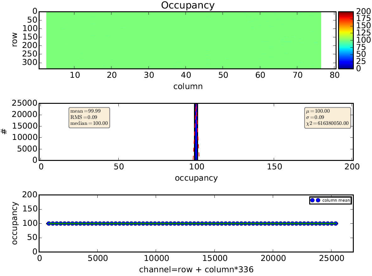
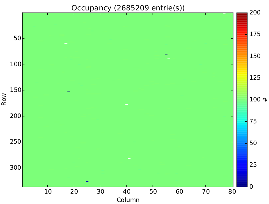
The occupancy per pixel and scan parameter is also plotted with a 2D heat map with logarithmic color coding. The data of a threshold scan is show in the following plot with scan parameter == PlsrDAC.

- HistThreshold: A two dimensional histogram (col x row) storing the threshold of each pixel. The threshold is given in pulser DAC and in electrons. For the conversion to electrons the PlsrDAC calibration values (offset + slope) in the config file are used.

- HistNoise: A two dimensional histogram (col x row) storing the noise of each pixel. The noise is given in pulser DAC and in electrons. For the conversion to electrons the PlsrDAC calibration slope in the config file is used.

- HistRelBcid: A one dimensional histogram [0:16[ storing the relative BCID of the hits.

- HistTot: A one dimensional histogram [0:16] storing the tot codes of the hits.

- HistErrorCounter: A one dimensional histogram [0:16] counting the event error codes that occured in events.

The error codes are:- No error (error code 0)
- Service record occurred in the event (1). This can happen if service records are activated and does not mean that there is a serious error. One should check the service record error code if this occurs to often.
- There is no external trigger (2). Usual case if no TLU is used.
- The LVL1 ID is not constant during the event (4). Serious error that should not be ignored. Indicates a bad Front-End / power-up.
- The number of BCIDs in the event is wrong (8). Serious error that should not be ignored.
- The event has at least one unknown word (16). Should not happen in normal operation mode (reasonable threshold, no noisy pixels). Serious error if occuring too often.
- The BCID counter is not increasing by one between two data headers (32). Error that may be ignored. Indicates a bad power-up. Power cycling usually helps.
- The event is externally triggered and a trigger error occured (64). Please contact the pyBAR developers if you see this.
- The software buffers are too small to store all hits of one event. The event is truncated (128). This indicates that there are too many data headers for TLU triggered events or too many hits per event for the analysis (__MAXHITBUFFERSIZE = 4000000). More than __MAXHITBUFFERSIZE per event is extreme and can only be created in very rare use cases (e.g. stop-mode readout).
- The event has one TDC word. Is expected if the FPGA TDC is used.
- The event more than one TDC word. Is expected if the source is very hot. These events cannot be used for TDC analysis. Thus there should be only a few events with more than one TDC word.
- The TDC value is too big and therefore meaningless.
- HistOcc: The occupancy histogram stores the FE hits for each scan parameter in a three dimensional map. The first two dimensions reflect the pixel alignment (col x row) and the third dimension is the scan parameter.
- HistTriggerErrorCounter: A one dimensional histogram [0:8] counting the trigger error codes that occured in events.

The error codes are:- No error (error code 0)
- Trigger number does not increase by 1 (1)
- One event has two trigger number words (2)
- Not used (4)
- Not used (8)
- Not used (16)
- HistServiceRecord: A one dimensional histogram [0:32] counting the service record codes that occured in events.
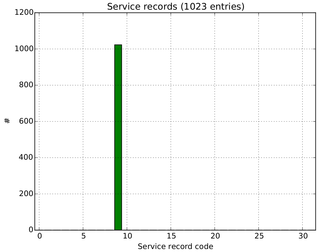
Please check the FE manual for error code explanations.
Clustered data is usually stored as additional nodes in the analyzed data file or in a new file. The nodes are cluster hits, cluster or histograms.
-
Cluster hits
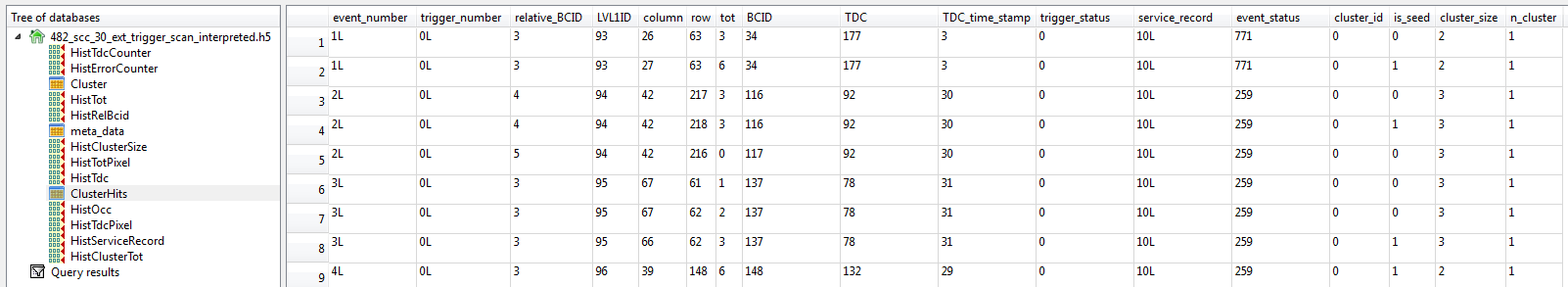
The table ClusterHits is a copy of the Hits table (see above) but with four additional columns:- cluster_id: The cluster ID of the hit [0:number of cluster in the event]
- is_seed: Is one if the hit is the seed hit, otherwise 0.
- cluster_size: The size of the cluster the hit belongs to.
- n_cluster: The number of cluster of the event the hit belongs to.
-
Cluster
The table Cluster stores the infos for each cluster.

The columns are:- event_number: The absolute event number. Only events with cluster appear here.
- id: The cluster ID of the cluster [0:number of cluster in the event].
- size: The number of hits that belong to the cluster.
- tot: The tot sum of all hits.
- charge: The charge sum of all hits (not used yet).
- seed_column: The column of the seed pixel.
- seed_row: The row of the seed pixel.
- event_status: The status of the event of the cluster. The event error code is a sum of the different binary coded event error codes that occured during the event. Please take a look at the histogram section for the error code explenation.
-
Cluster Histograms
Different histograms can be created on the fly while interpreting the data. Usually single cluster information are not needed while the cluster histograms provide sufficient information. The different histograms are:- HistClusterSize: A one dimensional histogram [0:1024] filled with the cluster sizes.

- HistClusterTot: A two dimensional histogram (tot x cluster size) storing the size of the cluster for different tot values. The cluster size = 0 column is the sum of the other columns.
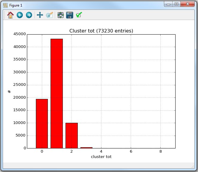
- HistClusterSize: A one dimensional histogram [0:1024] filled with the cluster sizes.
PyBAR has a real time online monitor that displays the data which is stored during a scan. The online monitor runs in a seperate process and does not influence the data taking. The online monitor can be opened and closed at any time.
Execute the online_monitor.py script from the pybar folder:
python online_monitor.py
A window will open:

Keep the right mouse button pressed to zoom in and out. You can switch between the plots by pressing on the blue tabs. Reorder the window by dragging the tabs.
The top right number is adjusting the integration time which is given in numbers of readout cycles. 0 means infinite integration time, 1 means a redraw for every readout, 2 a redraw for every other readout, …
To enable the online monitor for all run scripts, add the following lines to the configuration.yaml:
run_conf:
    send_data : 'tcp://127.0.0.1:5678'
The address tcp://127.0.0.1:5678 is the localhost with port 5678. Change this address to tcp://0.0.0.0:5678 to allow incoming connections on all interfaces. The online monitor script online_monitor.py can even run on another host. Changing the remote IP (default is localhost) of the online monitor needs the following command:
python online_monitor.py tcp://remote_ip:5678Note: On some operating systems, the firewall needs to be set up properly to allow using the online monitor over network.
Note: To display the data from an existing data output file, examine the replay_data.py script.
If the histograms mentioned above are not sufficient and there is no special analysis script in /pybar/scans or no fitting method in analysis.py that does what you want (like analyze_source_scan_tdc_data or def analyze_hits_per_scan_parameter) well… than you have to do your analysis on your own. The following sections explain the analysis details.
The pyBAR readout is designed in a way that every data word from the Front-End is stored and analyzed. There is no data reduction done in the FPGA, the user is in full control. Since the amount of data words can be large (e.g. threshold scan: 15000000 words = 450 Mb data) fast and optimized c++ classes were written to cope with the data efficiently. These classes are compiled via cython and all needed functions are wrapped in one python class called AnalyzeRawData. This class was written to hide the complexity of the conversion process. Additional helper function for the analysis are in analysis_utils. The compiled C++ code used in the background is intended to work and not to be changed on a frequent basis. To analyze the raw data is straight forward. An example script can be found here.
Warning the following section is only for interested people and does not have to be understood to do a self written analysis:
There are three objects in the AnalyzeRawData class for data analysis:
- PyDataInterpreter:
The PyDataInterpreter takes the raw data words (see data structures → Scan data file → raw data) and interprets them. This includes hit and event finding as well as error checks on the raw data structure and the counting of service records. For more information on the FE-I4 data structure please take a look at the FE manual. - PyDataHistograming:
The PyDataHistograming takes the hit infos from the PyDataInterpreter and histograms them. It also provides a fast algorithm to deduce the threshold and the noise from the occupancy data without S-Curve fitting. - PyDataClusterizer:
The PyDataClusterizer takes the hit and event infos from the PyDataInterpreter and clusters them.
A in depth view what the three different classes (PyDataInterpreter, PyDataHistograming,PyDataClusterizer) do and the input/output of the AnalyzeRawData shows the following figure.

The run scripts are located in the scans folder. Each run script contains a class, which is inherited from Fei4RunBase class (see fei4_run_base module).
Each script is a series of successive steps which are executed one after another. Inside each run script, 3 major methods needs to be defined:
- configure():
The DUT (readout hardware) and FE-I4 is initialized just before this step. In configure(), additional FE-I4 registers are programmed so that the scan step will work. The configuration is restored after scan step. - scan():
This function implements the scan algorithm. Usually, the data taking is started and stopped during the scan step. Also setting up of the DUT (readout hardware) will take place during this step. - analyze():
The analysis of the raw data will happen here. Usually, configuration changes are applied here. The configuration is stored just after the analyze step.
The following is a short summary of existing run scripts:
-
HitOR Calibration
HitOR calibration scan that calibrates the TDC for measuring the high precision charge spectrum using the TDC method. -
PlsrDAC Calibration
PlsrDAC calibration scan that measures the offset, slope and saturation voltage of the PlsrDAC for each double column (DC). -
Transient PlsrDAC Calibration
PlsrDAC calibration scan that measures the transient slope of the PlsrDAC for each double column by using an oscilloscope. -
ToT Calibration
ToT calibration scan that calibrates the ToT for measuring the charge spectrum using the ToT method. -
Analog Scan
Scan that uses analog injections to generate hits. -
Crosstalk Scan
Detecting crosstalk between pixels by injecting into neighbour pixels (long edge). -
Digital Scan
Scan that uses digital injections to generate hits. -
External Trigger Scan with EUDAQ
Source scan that uses trigger coming from EUDAQ TLU and connects with EUDAQ telescope software. -
External Trigger Scan
Source scan that uses external trigger. HitOR/TDC method for high precision charge measurements can be enabled. -
External Trigger Scan with GDAC
Source scan that uses external trigger for triggering and sweeps the GDAC (global threshold). This scan is used for threshold method to measure the charge spectrum. -
External Trigger Stop Mode Scan
Source scan that uses external trigger for triggering and puts the FE-I4 into stop mode to read out up to 255 bunch crossings. Note that the trigger rate is limited. -
FE-I4 Self-Trigger Scan
Source scan that uses FE-I4 HitOR/HitBus for self-triggering. -
Hit Delay and Timewalk Scan
Measuring the pixel-by-pixel hit delay and timewalk scan by using the internal pulser (PlsrDAC). -
Init Scan
Scan that writes the configuration into the FE-I4. -
Threshold Scan
Threshold scan to measure the threshold and noise distribution. The threshold mean and noise are plotted in PlsrDAC and electrons. The conversion to electrons is done by taking the slope and offset of the linear PlsrDAC transfer function and the injection capacitance values (Q = C * dV(PlsrDAC)). The slope and offset of the PlsrDAC transfer function V(PlsrDAC) are measured in the calibrate PlsrDAC scan and are stored in the global config file. -
Fast Threshold Scan
A faster version of the threshold scan by automatic detection of the start and stop of the S-curve. The threshold mean and noise are plotted in PlsrDAC and electrons. The conversion to electrons is done by taking the slope and offset of the linear PlsrDAC transfer function and the injection capacitance values (Q = C * dV(PlsrDAC)). The slope and offset of the PlsrDAC transfer function V(PlsrDAC) are measured in the calibrate PlsrDAC scan and are stored in the global config file. -
Register Test
A FE-I4 global and pixel register test. Also reads back FE-I4 serial number. -
TDC Test
Debugging and testing functionality of TDC (linearity of TDC counter and trigger distance counter). -
Pixel Feedback Tuning
Tuning of the pixel feedback current (FDAC). -
Global Feedback Tuning
Tuning of the global feedback current (PrmpVbpf). -
Tune FE-I4
Meta script that does the full tuning (VthinAlt_Fine, TDAC, PrmpVbpf, FDAC). -
Global Threshold Tuning
Tuning of the global threshold (GDAC/VthinAlt_Fine). -
Hot Pixel Tuning
Masking hot pixels which are usually not seen by the Noise Occupancy Scan. The scan uses FEI4 self-trigger mode for highest detection sensitivity. -
Merged Pixel Masking
Detecting conductive interconnection between pixels and mask them. -
Noise Occupancy Scan
Masking noisy/hot pixels by sending LVL1 triggers to the FE-I4. -
Stuck Pixel Scan
Masking stuck-high (e.g. preamp always high) pixels. -
Pixel Threshold Tuning
Tuning of the pixel threshold (TDAC). -
Threshold Baseline Tuning
Measuring pixel noise occupancy to tune to lowest possible threshold.
Note: more documentation is available inside each run script.
Creating a pyBAR test environment is is useful in the following scenarios:
- testing a large number of modules
- testing multiple modules in parallel, which are connected to different readout boards (e.g. test beam, module qualification)
- the module data should be stored somewhere else than the pyBAR project folder
- you want to keep all configuration files and module data in a safe place
The following steps show how to create a pyBAR test environment. Repeat the steps for each readout board:
- Create a new folder somewhere on your hard drive.
Give the folder a descriptive name (e.g. module name).
Note: please check if enough free memory is available (several GB per module). - Copy the pyBAR configuration file (configuration.yaml), the DUT configuration file (e.g. dut_mio.yaml), and the DUT initialization configuration file (e.g. dut_configuration_mio.yaml) to the newly created folder.
Change the configuration files as usual. - Create your own run script and place it into the newly created folder. The script should use the pyBAR run manager to execute the pyBAR run scripts.
Note: A more detailed example on how to use the run manager is given here.from pybar import * runmngr = RunManager('configuration.yaml') runmngr.run_run(run=AnalogScan) - Another way to execute the run scripts is to use an interactive shell (e.g. IPython). To start IPython, change to the newly created folder and type
ipythoninto the shell. To run a run, copy the above listing line by line.
Note: runconda install ipythonto install IPython.
A full FE-I4 tuning (VthinAlt_Fine, TDAC, PrmpVbpf, FDAC) takes usually less than 5 minutes per FE-I4 chip. The tuning is implemented in the tune_fei4.py meta script.
To setup the tuning parametes (e.g. threshold, gain), different methods are available:
- Change the
_default_run_confinside the tune_fei4.py file. - Adding run configuration to the configuration.yaml:
Fei4Tuning: enable_shift_masks : ["Enable", "C_Low", "C_High"] target_threshold : 50 # target threshold target_charge : 280 # target charge target_tot : 5 # target ToT global_iterations : 4 local_iterations : 3 - Via pyBAR run manager:The output PDF contains all the information if the tuning was successful. To verify the ToT-to-Charge (gain) calibration use scan_analog.py and to verify the threshold calibration use scan_threshold.py.
from pybar.run_manager import RunManager
from pybar.scans.tune_fei4 import Fei4Tuning
if __name__ == "__main__":
    runmngr = RunManager('configuration.yaml')
    status = runmngr.run_run(run=Fei4Tuning, run_conf={"enable_shift_masks": ["Enable", "C_Low", "C_High"], "target_threshold": 50, "target_charge": 280, "target_tot": 5, "global_iterations": 4, "local_iterations": 3})
    print 'Status:', status
Note:
- To mask any noisy/hot pixels, execute tune_noise_occupancy.py and tune_stuck_pixel.py (with default parameters).
- A tuning script that uses the run manager is given here.
The external trigger scan in scan_ext_trigger.py can be used for the following scenarios:
- TLU trigger via RJ45/TLU port
- Any single ended signal (e.g. amplified scintillator signal, FE-I4 HitOR signal)
The trigger input has to be set up inside the Basil initialization configuration (e.g. dut_configuration_mio.yaml).
TLU:
    TRIGGER_MODE        : 0
    TRIGGER_SELECT      : 0
    TRIGGER_INVERT      : 0
TRIGGER_VETO_SELECT : 255-
TRIGGER_MODE
Selcting trigger mode, e.g. 0: single ended trigger inputs, 4: TLU data handshake mode. -
TRIGGER_SELECT
Selecting the trigger input (up to 8 input channels). Trigger inputs are used inTRIGGER_MODE0 only. 0 means all inputs disabled, 255 means all inputs activated. -
TRIGGER_INVERT
Inverting selected trigger input. -
TRIGGER_VETO_SELECT
Selecting the veto input (up to 8 input channels). 0 means all inputs disabled, 255 means all inputs activated. It is recommended to keep default setting (255).
Note:
- The trigger input select may depend on the FPGA implementation. More hints are given inside the Basil initialization configuration (e.g. dut_configuration_mio.yaml).
The pin assignment of the boards is documented here. - Additional run script parameters (e.g. max trigger, timeouts, trigger rate limit) are documented inside scan_ext_trigger.py.
- More information on the FPGA firmware module is available in the Basil documentation.
You can use additional lab devices after you have specified them in the hardware configuration file, that describes your hardware system (e.g. dut_mio.yaml). To add a lab device you have to specify its driver in the hw_drivers section and the way how it is connected in the transfer_layer. Assuming you want to use a Keythley 2410 Sourcemeter you have to add in the
hw_drivers section:
hw_drivers:
  - name      : Sourcemeter
    type      : scpi
    interface : Visa
    init      :
        device  : Keithley 2410
        timeout : 1
and if it is connected via GPIB in the transfer_layer:
transfer_layer:
  - name     : Visa
    type     : Visa
    init     :
        resource_name : GPIB0::12::INSTR
h2. Advanced Scans and Analysis
For some special applications you might find our Application Notes useful.